Take-Home Exercise 03

1. Overview

With reference to the Mini-Challenge 3 of VAST Challenge 2023 and by using visual analytics to understand the patterns of groups in the knowledge graph and highlight anomalous groups.

1.1. The Task

Use visual analytics to identify anomalies in the business groups present in the knowledge graph.

1.2. Data Source

For this task, we will make use of the MC3.json provided for the data analysis and visualisation.

2. Loading and Launching of Required R Packages

The required R library packages are being loaded. For this exercise, we will make use of the following R library packages.

• jsonlite, JSON parser and generator optimized for statistical data and the web.
• tidygraph provides a tidy framework for all things relational (networks/graphs, trees, etc.)
• ggraph, an extension of the ggplot2 API tailored to graph visualizations and provides the same flexible approach to building up plots layer by layer.
• visNetwork for network visualization.
• tidyverse, a family of modern R packages specially designed to support data science, analysis and communication task including creating static statistical graphs.
• tidytext for text mining and conversion of text to and from tidy formats.
• skimr provides summary statistics about variables in data frames, tibbles, data tables and vectors.
• DT provides an R interface to the JavaScript library DataTables that create interactive table on html page.
• treemap for plotting static treemap.
• treemapify provides ‘ggplot2’ geoms for drawing treemaps.
• igraph for creating and manipulating graphs and analyzing networks.
• plotly for creating interactive web-based graphs via the open source JavaScript.

The code chunk below uses pacman::p_load() to check if the above packages are installed. If they are, they will be loaded into the R environment.

Code

pacman::p_load(jsonlite, tidygraph, ggraph, visNetwork, skimr,
               tidyverse, graphlayouts, ggforce, DT, tidytext,
               treemap, treemapify, igraph, plotly)

3. Data Preparation & Initial Analysis

We will first load each of the data files into the environment and perform data wrangling.

3.1. Loading and Extracting the Data

Based on the VAST 2023 data notes, column dataset will always be ‘mc3’, to represent this set of data belongs to mini challenge 3. As such, we will not import this column into the R environment.

3.1.1. Load main file MC3.json

We will first load in the main file, MC3.json, then extract the nodes and edges (links) information out.

Code

mc3_data <- fromJSON("data/MC3.json")

3.1.1.1. Extracting the nodes data.frame from MC3

We will first extract the nodes info from mc3_data.

Code

mc3_nodes_raw <- as_tibble(mc3_data$nodes) %>%
  select(id, country, type, product_services, revenue_omu)

Then we will mutate the data by converting id, country, type and product_services into character data type, while revenue_omu will be converted to numeric data type. We will also rearrange the columns by using select().

Code

mc3_nodes_raw <- mc3_nodes_raw %>%
  mutate(country = as.character(country),
         id = as.character(id),
         product_services = as.character(product_services),
         revenue_omu = as.numeric(as.character(revenue_omu)),
         type = as.character(type)) %>%
  select(id, country, type, revenue_omu, product_services)

3.1.1.2. Extracting the edges (links) data.frame from mc3

Next, we will extract the edges info from mc3_data.

Code

mc3_edges_raw <- as_tibble(mc3_data$links) %>%
  select(source, target, type)

Then we will mutate the data by converting source, target and type into character data type. At the same time, we will compute the weights of the edges.

Code

mc3_edges_raw <- mc3_edges_raw %>%
  distinct() %>%
  mutate(source = as.character(source),
         target = as.character(target), 
         type = as.character(type)) %>%
  group_by(source, target, type) %>%
  summarise(weights = n()) %>%
  filter(source != target) %>%
  ungroup()

3.1.1.3. Examining the structure of mc3_edges_raw

Code

skim(mc3_edges_raw)

Data summary

Name	mc3_edges_raw
Number of rows	24036
Number of columns	4
_______________________
Column type frequency:
character	3
numeric	1
________________________
Group variables	None

Variable type: character

skim_variable	n_missing	complete_rate	min	max	empty	n_unique	whitespace
source	0	1	6	700	0	12856	0
target	0	1	6	28	0	21265	0
type	0	1	16	16	0	2	0

Variable type: numeric

skim_variable	n_missing	complete_rate	mean	sd	p0	p25	p50	p75	p100	hist
weights	0	1	1	0	1	1	1	1	1	▁▁▇▁▁

Examination of the data structure

The report above reveals that there is no missing values in all fields in mc3_edges_raw.

However, the source field has a maximum value of 700 (in lexicographic order), which seemed a little to lengthy, as compared to the target field which only has a maximum value of 28. With that, we will take a closer look at the data under the source field.

3.1.1.4. Examining the data distribution of mc3_edges_raw

Source Field

We will take a closer look at the source field to investigate the reason of having a maximum value of 700 by counting the frequency of each unique value and take a peep of the actual value by listing the first 20 records to detect any anomalies in the data. We will list the string values in descending order based on its frequency.

Code

mc3_edges_raw_source_freq <- mc3_edges_raw %>%
  group_by(source) %>%
  summarise(freq_cnt = n()) %>%
  arrange(desc(freq_cnt)) %>%
  ungroup()

head(mc3_edges_raw_source_freq, 20)

# A tibble: 20 × 2
   source                                                      freq_cnt
   <chr>                                                          <int>
 1 "Vespuci Sandbar Sp Brothers"                                    120
 2 "Dutch Oyster Sagl Cruise ship"                                   91
 3 "Niger Bend   AS Express"                                         72
 4 "Ola de la Costa N.V."                                            65
 5 "Wave Warriors S.A. de C.V. Express"                              62
 6 "Caracola del Este Enterprises"                                   54
 7 "Bahía de Plata Submarine"                                        49
 8 "BlueTide GmbH & Co. KG"                                          49
 9 "Brisa del Mar Current Inc Express"                               49
10 "Luangwa River   Limited Liability Company Holdings"              49
11 "Congo Rapids   Ltd. Corporation"                                 48
12 "Mar del Golfo Ges.m.b.H. Transport"                              48
13 "Ocean Quest S.A. de C.V."                                        48
14 "Victoria Falls   OJSC & Son's"                                   46
15 "Tamil Nadu s NV Merchants"                                       42
16 "Aqua Aura SE Marine life"                                        41
17 "Indian Ocean Harvesters S.A. de C.V. Consultants"                41
18 "Rufiji Delta  GmbH Express"                                      40
19 "c(\"The Sea Turtle Company\", \"The Sea Turtle Company\")"       39
20 "The Salted Pearl Inc Pelican"                                    38

Examination of the ‘source’ field

The results revealed that there were lists (denoted by c() embedded within the source field, as indicated in the screenshot below.

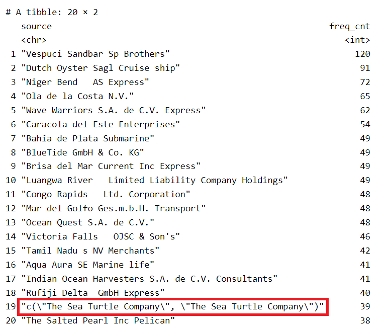
We will have to break these lists further into single values before deriving the weight of the edges.

Firstly, we will have to extract all the records that contain an embedded list in the source field. We will make use of the substr() method to identify these records.

Code

mc3_edges_list_in_source <- mc3_edges_raw %>%
  filter(substr(source, 1, 2) %in% "c(") %>%
  ungroup()

mc3_edges_list_in_source

# A tibble: 2,169 × 4
   source                                                   target type  weights
   <chr>                                                    <chr>  <chr>   <int>
 1 "c(\"1 Ltd. Liability Co\", \"1 Ltd. Liability Co\")"    Yesen… Comp…       1
 2 "c(\"1 Swordfish Ltd Solutions\", \"1 Swordfish Ltd Sol… Danie… Comp…       1
 3 "c(\"5 Limited Liability Company\", \"Bahía de Coral Kg… Britt… Bene…       1
 4 "c(\"5 Limited Liability Company\", \"Bahía de Coral Kg… Eliza… Bene…       1
 5 "c(\"5 Limited Liability Company\", \"Bahía de Coral Kg… Sandr… Comp…       1
 6 "c(\"5 Oyj Marine life\", \"Náutica del Sol Kga\")"      Rober… Comp…       1
 7 "c(\"6 GmbH & Co. KG\", \"6 GmbH & Co. KG\", \"6 GmbH &… Moniq… Comp…       1
 8 "c(\"7 Ltd. Liability Co Express\", \"7 Ltd. Liability … Cassi… Bene…       1
 9 "c(\"7 Ltd. Liability Co Express\", \"7 Ltd. Liability … Dawn … Bene…       1
10 "c(\"7 Ltd. Liability Co Express\", \"7 Ltd. Liability … Hanna… Comp…       1
# ℹ 2,159 more rows

Examination of type field

A total of 2,169 records were found to contain embedded list of entities in the source field. We will have to break up the individual list using unnest() and put these individual entities into the source field.

Break up the Individual List

The following code chunk will break up the individual list using unnest() and put these individual entities into the source field.

We will also remove:

• leading/trailing whitespace and empty values using trimws()
• double quotes using gsub()
• values that only contain the character, c

We will then recompute the weights based on the extracted entities, grouping them by source, target and type.

Code

# Break up values containing lists using unnest().
# It will split the string when it encounters the open parenthesis "(",
# comma "," and close parenthesis ")" 
broken_source <- unnest(mc3_edges_list_in_source, 
                        source = strsplit(as.character(source),
                                          "\\(|\\,|\\)"))

# Remove leading/trailing whitespace and also filter records with only
# the character "c" as the source
broken_source <- broken_source %>%
  mutate(source = gsub("\"", "", source)) %>%
  filter(source != "c") %>%
  mutate(source = trimws(source)) %>%
  mutate(target = trimws(target)) %>%
  group_by(source, target, type) %>%
  summarise(weights = n()) %>%
  filter(source != target) %>%
  distinct() %>%
  ungroup()

Combining the list of entries with the rest of the mc3_edges_raw

Now that we have extracted the list of entities (broken_source), we will combine the list with mc3_edges_raw that do not have the embedded list (i.e. mc3_edges_nolist) and study the data.

In order to create mc3_edges_nolist, we will make use of filter() and substr() to identify those records that do not start with "c(". this will help to filter off those records that have the embedded list in the source field.

Once we combine the 2 lists, we will do a thorough cleaning to ensure that there is no leading/trailing white spaces in all the 3 fields by using trimws(). At the same time, we will remove any duplicate records present and arrange the list in descending order based on the weights field.

Code

# Extract the list of records without the embedded list in source field
mc3_edges_nolist <- mc3_edges_raw %>%
  filter(!substr(source, 1, 2) %in% "c(") %>%
  distinct() %>%
  ungroup()

# Merge the extracted entities (broken_source) to the list
final_mc3_edges <- rbind(mc3_edges_nolist, broken_source) 

# Clean up the combined list
final_mc3_edges <- final_mc3_edges %>%
  mutate(source = trimws(source)) %>%
  mutate(target = trimws(target)) %>%
  mutate(type = trimws(type)) %>%
  group_by(source, target, type) %>%
  filter(source != target) %>%
  distinct() %>%
  arrange(desc(weights)) %>%
  ungroup()

datatable(final_mc3_edges,
          class="stripe",
          caption = "\nTable 1: List of Entities\n",
          colnames = c("Source", "Target", "Type", "Weights"),
          options = list(
            columnDefs = list(list(className = 'dt-center',
                                   targets="_all"))))

Observations from Table 1

Table 1 revealed that there are some of the individuals have multiple linkages to the same company, which we will need to probe further in order to understand the underlying relationships.

In addition, we also noticed that there are some individuals that included salutations (i.e. Dr., Mr., Ms. and Mrs.), as part of their names. As we do not have additional information to determine whether similar names with salutations and without salutations are referring the the same individual, we will have to treat them differently. Hence, as part of data discovery, we will flag this as a data quality issue.

3.1.1.5. Understanding the Relationships between Company, Beneficial Owner and Company Contacts

In this section, we will find out about the relationships between Company, Beneficial Owner and Company Contacts:

• From Company Perspective:

  • 1. Number of Beneficial Owners
  • 2. Number of Company Contacts

• From Individual Person Perspective:

  • 1. Number of Companies A Person Owns
  • 2. Number of Companies A Person is Contact

3.1.1.5.1. From Company Perspective

Number of Beneficial Owners Per Company

Code

# Derive the number of beneficial owners that a company has
final_mc3_edges_coy_bo_count <- final_mc3_edges %>%
  group_by(source) %>%  
  filter(type == "Beneficial Owner") %>%
  summarise(coy_bo_count = n()) %>%
  distinct() %>%
  arrange(desc(coy_bo_count)) %>%
  ungroup()

datatable(final_mc3_edges_coy_bo_count,
          class="stripe",
          caption = "\nTable 2: Number of Beneficial Owners by Company\n",
          colnames = c("Company", "Beneficial Owner Count"),
          options = list(
            columnDefs = list(list(className = 'dt-center',
                                   targets="_all"))))

Number of Company Contacts Per Company

Code

# Derive the number of company contacts that a company has
final_mc3_edges_coy_cc_count <- final_mc3_edges %>%
  group_by(source) %>%  
  filter(type == "Company Contacts") %>%
  summarise(coy_cc_count = n()) %>%
  distinct() %>%
  arrange(desc(coy_cc_count)) %>%
  ungroup()

datatable(final_mc3_edges_coy_cc_count,
          class="stripe",
          caption = "\nTable 3: Number of Contacts by Company\n",
          colnames = c("Company", "Company Contacts Count"),
          options = list(
            columnDefs = list(list(className = 'dt-center',
                                   targets="_all"))))

Observations from Table 2 and Table 3

Table 2 revealed that there are a number of companies that have multiple beneficial owners. For the purpose of analysis, we will focus on the companies with more than 50 beneficial owners.

Table 3 revealed that there are a number of companies that have multiple company contacts, with “Aqua Aura SE Marine life” having the highest number of 11 company contacts. For the purpose of analysis, we will focus on the companies that have more than 5 company contacts.

3.1.1.5.2. From Individual Person Perspective

Number of Company that an Individual Owns (Beneficial Owner)

Code

# Derive the number of companies that an individual owns
final_mc3_edges_ind_bo_count <- final_mc3_edges %>%
  group_by(target) %>%  
  filter(type == "Beneficial Owner") %>%
  summarise(ind_bo_count = n()) %>%
  distinct() %>%
  arrange(desc(ind_bo_count)) %>%
  ungroup()

datatable(final_mc3_edges_ind_bo_count,
          class="stripe",
          caption = "\nTable 4: Number of Companies that an Individual Owns (Beneficial Owner)\n",
          colnames = c("Person", "Company Count"),
          options = list(
            columnDefs = list(list(className = 'dt-center',
                                   targets="_all"))))

Number of Company that an Individual is Company Contact

Code

# Derive the number of companies that an individual is Company Contact
final_mc3_edges_ind_cc_count <- final_mc3_edges %>%
  group_by(target) %>%  
  filter(type == "Company Contacts") %>%
  summarise(ind_cc_count = n()) %>%
  distinct() %>%
  arrange(desc(ind_cc_count)) %>%
  ungroup()

datatable(final_mc3_edges_ind_cc_count,
          class="stripe",
          caption = "\nTable 5: Number of Companies that an Individual is Company Contact\n",
          colnames = c("Person", "Company Count"),
          options = list(
            columnDefs = list(list(className = 'dt-center',
                                   targets="_all"))))

Analysis from Table 4 and Table 5

From Table 4 above, it confirmed that there are a number of individuals who own more than 1 company.

From Table 5 above, it confirmed that some of the individuals are Company Contacts for multiple companies.

3.1.2. Initial Network Visualisation & Analysis

We will start to perform some initial analysis based on the information that we gathered so far.

3.1.2.1. Visualising From Company’s Perspective

Compiling the list of Individuals with reference to the Companies

From the results in Table 2 (Number of Beneficial Owners by Company) and Table 3 (Number of Contacts by Company) above, we will extract out the respective companies that have a high number of beneficial owners and company contacts. Then we will gather the individuals’ information from mc3_nodes_raw.

We will perform the following steps to get the list of unique companies:

• Retrieve the list of companies from final_mc3_edges_coy_bo_count for those companies that have more than 50 beneficial owners, using the filter().
• Retrieve the list of companies from final_mc3_edges_coy_cc_count for those companies that have more than 5 company contacts, using the filter().
• Combine both the above lists by extracting out the matching records from the final_mc3_edges dataframe.

Code

coy_bo_above_50 <- final_mc3_edges_coy_bo_count %>%
  filter(coy_bo_count >= 50) 

coy_cc_above_5 <- final_mc3_edges_coy_cc_count %>%
  filter(coy_cc_count >= 5)

# Combining the list of companies are linked to the individuals
coy_to_ind_mc3_edges <- final_mc3_edges %>%
  filter(source %in% coy_bo_above_50$source |
           source %in% coy_cc_above_5$source) %>%
  distinct()

Once we have the unique list of companies and the individuals, we will then form the nodes dataframe.

Design Consideration

In order to easily identify whether a node is a Company, Beneficial Owner or Company Contacts, we will include a group attribute in the nodes dataframe. We will make use of case_when() functions to build the conditions in determining the value of group for each node. The conditions are as follows:

• If the id can be found in the source field of coy_to_ind_mc3_edges, then the node is a Company (i.e. group = “Company”)
• Otherwise, if the id is found in the target field of coy_to_ind_mc3_edges, we will then need to check the type field of coy_to_ind_mc3_edges to determine whether the node is Beneficial Owner or Company Contacts.

Code

# Forming the nodes from the combined_sources
id1_coy <- coy_to_ind_mc3_edges %>%
  select(source) %>%
  rename(id = source)

id2_coy <- coy_to_ind_mc3_edges %>%
  select(target) %>%
  rename(id = target)

# create a new nodes data table derived from the source and target of edge data. This would ensure that only nodes with connections will be included.
coy_to_ind_mc3_nodes <- rbind(id1_coy, id2_coy) 

# Adding a group attribute, into the nodes dataframe, to differentiate whether the node is a Company, Beneficial Owner or Company Contacts. 
coy_to_ind_mc3_nodes <- coy_to_ind_mc3_nodes %>%
  mutate( group = case_when(
    id %in% coy_to_ind_mc3_edges$source ~ "Company",
    id %in% coy_to_ind_mc3_edges$target & 
      coy_to_ind_mc3_edges$type == "Beneficial Owner" ~ "Beneficial Owner",
    id %in% coy_to_ind_mc3_edges$target & 
      coy_to_ind_mc3_edges$type == "Company Contacts" ~ "Company Contacts"
    )
  )

Building the tbl_graph object for visualisation

We will build up the tbl_graph object in preparation to visualise the Company-Individual Relationship.

Code

# Build tbl_graph using the valid nodes and edges 
coy_to_ind_graph <- tbl_graph(nodes = coy_to_ind_mc3_nodes,
                              edges = coy_to_ind_mc3_edges,
                              directed = FALSE)

# Renaming the id column to label and
# create a new column, id with the row_number()
coy_to_ind_graph <- coy_to_ind_graph %>%
  activate(nodes) %>%
  rename(label = id) %>%
  mutate(id=row_number())

# Converting the nodes into a tibble dataframe
coy_to_ind_nodes_df <- coy_to_ind_graph %>%
  activate(nodes) %>%
  as_tibble() 

# Converting the edges into a tibble dataframe
coy_to_ind_edges_df <- coy_to_ind_graph %>%
  activate(edges) %>%
  as_tibble()

Visualisation of the Relationship of Company to Individual

Design Consideration

1. We will make use of the group attribute that we created in the earlier section to clearly identify the different types of nodes (Company, Beneficial Owner, Company Contacts).
2. For the ease of selecting a particular entity, a dropdown list with all the entities (nodes) present in the graph is provided. The list is also sorted in ascending order by using arrange().
3. Mouse pointer hover action is also included on the graph so that the user can hover the mouse pointer over the graph to look at the possible different ‘groups’ of connectivity.

Code

# Preparing the data for visualisation
nodes <- coy_to_ind_nodes_df %>%
  filter(id %in% c(coy_to_ind_edges_df$from,
                   coy_to_ind_edges_df$to)) %>%
  arrange(label)

# Building the network graph using visNetwork package
vis_nw <- visNetwork(nodes, 
                     coy_to_ind_edges_df,
                     main = "Relationship of Company to Individual") %>%
  visIgraphLayout(layout = "layout_with_fr") %>%
  visLayout(randomSeed = 1234) %>%
  visNodes(size = 30) %>%
  visOptions(highlightNearest = list(enabled = T, degree = 2, hover = T),
             nodesIdSelection = TRUE) %>%
  visLegend(width = 0.1, position = "right", main = "group") %>%  
  visEdges(smooth = list(enabled = TRUE, type = "curvedCW"))

vis_nw

Observations

From the network graph above, we are able to see the relationships of the companies that have significantly high number of owners (>= 50) and high number of company contacts (>= 5) as compared to the rest of the companies in the dataset.

It is observed that there are 5 Beneficial Owners (Blue-coloured nodes) that owned at least 2 of the companies in the network. These Beneficial Owners are:

• Jeremy Lee, owning Congo Rapids Ltd. Corporation and Niger Bends AS Express
• Randy Martinez, owning Caracola del Este Enterprises and Dutch Oyster Sagl Cruise ship
• James Thompson, owning Caracola del Este Enterprises and Wave Warriors S.A. de C.V. Express
• Dale Rhodes and Cynthia Murphy, owning both Irish Mackerel S.A. de C.V. Marine biology and Aqua Aura Se Marine Life

It is noted that Karen Martinez is also a Beneficial Owner of Irish Mackerel S.A. de C.V. Marine biology, which has a total of 7 Company Contacts.

We also noted that there are incidents of companies that have a significantly high number of company contacts,

• Kerala S.A. de C.V. Express, owned by Jennifer Abbott, has 5 company contacts
• Irish Mackerel S.A. de C.V. Marine biology, owned by Karen Martinez, Dale Rhodes and Cynthia Murphy, has a total of 7 Company Contacts.
• Smith Inc has 12 Beneficial Owners and 5 Company Contacts.

We will need to look out for the above-mentioned nodes in our subsequent analysis.

3.1.2.2. Visualising From Individual Person Perspective

Consolidating the list of Companies with reference to the Individuals with multiple companies

From the analysis results above, we will extract out the respective companies that these individuals are involved in. Then we will gather the company information from mc3_nodes_raw.

We will perform the following steps to get the list of unique companies:

• Retrieve the list of companies from final_mc3_edges_ind_bo_count for those individuals who owns more than 5 companies, using the filter().
• Retrieve the list of companies from final_mc3_edges_ind_cc_count for those individuals who are contacts for more than 4 companies, using the filter().
• Combine both the above lists by extracting out the matching records from the final_mc3_edges dataframe.

Code

ind_bo_above_5 <- final_mc3_edges_ind_bo_count %>%
  filter(ind_bo_count >= 5) 

ind_cc_above_4 <- final_mc3_edges_ind_cc_count %>%
  filter(ind_cc_count >= 4)

# Combining the list of companies are linked to the individuals
ind_to_coy_mc3_edges <- final_mc3_edges %>%
  filter(target %in% ind_bo_above_5$target == TRUE |
           target %in% ind_cc_above_4$target == TRUE) %>%
  distinct()

Once we have the unique list of companies, we will then form the nodes dataframe.

Design Consideration

In order to easily identify whether a node is a Company, Beneficial Owner or Company Contacts, we will include a group attribute in the nodes dataframe. We will make use of case_when() functions to build the conditions in determining the value of group for each node. The conditions are as follows:

• If the id can be found in the source field of ind_to_coy_mc3_edges, then the node is a Company (i.e. group = “Company”)
• Otherwise, if the id is found in the target field of ind_to_coy_mc3_edges, we will then need to check the type field of ind_to_coy_mc3_edges to determine whether the node is Beneficial Owner or Company Contacts.

Code

# Forming the nodes from the combined_sources
id1 <- ind_to_coy_mc3_edges %>%
  select(source) %>%
  rename(id = source)

id2 <- ind_to_coy_mc3_edges %>%
  select(target) %>%
  rename(id = target)

# create a new nodes data table derived from the source and target of edge data. This would ensure that only nodes with connections will be included.
ind_to_coy_mc3_nodes <- rbind(id1, id2) %>%
  distinct()

# Adding a group attribute, into the nodes dataframe, to differentiate whether the node is a Company, Beneficial Owner or Company Contacts. 
ind_to_coy_mc3_nodes <- ind_to_coy_mc3_nodes %>%
  mutate( group = case_when(
    id %in% ind_to_coy_mc3_edges$source ~ "Company",
    id %in% ind_bo_above_5$target ~ "Beneficial Owner",
    id %in% ind_cc_above_4$target ~ "Company Contacts"
    )
  )

Building the tbl_graph object for visualisation

We will build up the tbl_graph object in preparation to visualise the Company-Individual Relationship.

Code

# Build tbl_graph using the valid nodes and edges 
ind_to_coy_graph <- tbl_graph(nodes = ind_to_coy_mc3_nodes,
                              edges = ind_to_coy_mc3_edges,
                              directed = FALSE)

# Renaming the id column to label and
# create a new column, id with the row_number()
ind_to_coy_graph <- ind_to_coy_graph %>%
  activate(nodes) %>%
  rename(label = id) %>%
  mutate(id=row_number())

# Converting the nodes into a tibble dataframe
ind_to_coy_nodes_df <- ind_to_coy_graph %>%
  activate(nodes) %>%
  as_tibble() 

# Converting the edges into a tibble dataframe
ind_to_coy_edges_df <- ind_to_coy_graph %>%
  activate(edges) %>%
  as_tibble()

Visualisation of the Relationship of Individual to Company

Design Consideration

1. We will make use of the group attribute that we created in the earlier section to clearly identify the different types of nodes (Company, Beneficial Owner, Company Contacts).
2. For the ease of selecting a particular entity, a dropdown list with all the entities (nodes) present in the graph is provided. The list is also sorted in ascending order by using arrange().
3. Mouse pointer hover action is also included on the graph so that the user can hover the mouse pointer over the graph to look at the possible different ‘groups’ of connectivity.

Code

# Preparing the data for visualisation
nodes <- ind_to_coy_nodes_df %>%
  filter(id %in% c(ind_to_coy_edges_df$from,
                   ind_to_coy_edges_df$to)) %>%
  arrange(label)

# Building the network graph using visNetwork package
vis_nw <- visNetwork(nodes, 
                     ind_to_coy_edges_df,
                     main = "Relationship of Individual to Company") %>%
  visIgraphLayout(layout = "layout_with_fr") %>%
  visLayout(randomSeed = 1234) %>%
  visNodes(size = 30) %>%
  visOptions(highlightNearest = list(enabled = T, degree = 2, hover = T),
             nodesIdSelection = TRUE) %>%
  visLegend(width = 0.1, position = "right", main = "group") %>%  
  visEdges(smooth = list(enabled = TRUE, type = "curvedCW"))

vis_nw

Observations

From the network graph above, we are able to see the relationships of the individual Beneficial Owner/Company Contact to the companies that they have linked.

We can also see that there is a significantly network which comprised of 7 smaller clusters, as shown in the image below.

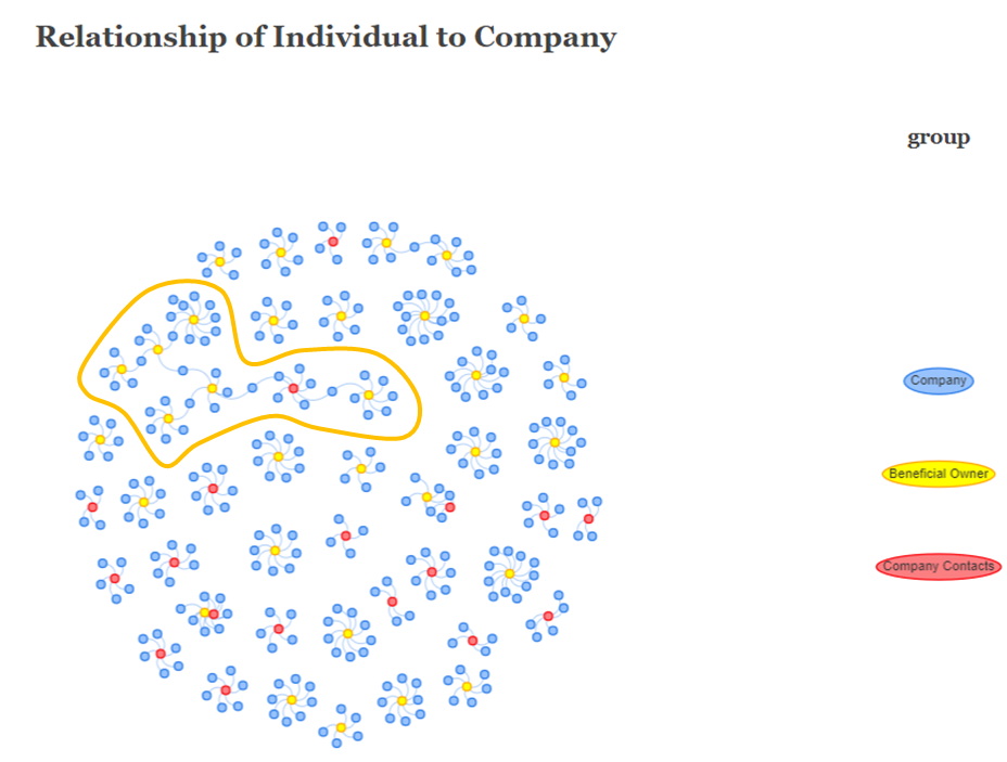
For the purpose of analysis, the labels of the connected nodes are listed below:

• Red-Coloured Node (Company Contacts): David Smith

• Yellow-Coloured Nodes (Beneficial Owner):

  • James Smith
  • Mary Williams
  • David Thomas
  • Jessica Brown
  • Michael Miller and
  • Jennifer Smith

• Blue-Coloured Nodes (Company):

  • Spanish Shrimp A/S Marine (between James Smith and David Smith)
  • Ocean Quest S.A. de C.V. (between David Smith and David Thomas)
  • Nagaland Sea Catch Ltd. Liability Co Logistics (between Mary Williams and David Thomas)
  • BlueTide GmbH & Co. KG (betweeen David Thomas and Jessica Brown)
  • West Fish GmbH Transport (between Jessica Brown and Michael Miller)
  • Mar del Oeste - (between Jessica Brown and Jennifer Smith)

We will need to look out for the above-mentioned nodes in our subsequent analysis.

3.2. Merging the information with mc3_nodes_raw

Firstly, we will make use of the setdiff() function to identify the values that are missing in mc3_nodes_raw. missing_source will contain all the values that are present in final_mc3_edges$source but not in mc3_nodes_raw$id.

We will then create a tibble dataframe, containing this list, in preparation to combine it with final_mc3_edges to form the eventual nodes dataframe for analysis.

As we do not have any information for country, revenue_omu and product_services fields, we will make use of NA_character_ and NA_real_ constants in R to pre-fill the missing values.

We will also perform the similar steps for final_mc3_edges$target.

Code

# Identify missing values in the 'source' column of 'final_mc3_edges'
missing_source <- setdiff(final_mc3_edges$source, mc3_nodes_raw$id) 

# Create a new dataframe for the missing 'source' values
missing_source_df <- tibble(
  id = missing_source,
  country = rep(NA_character_, length(missing_source)),
  type = rep("Company", length(missing_source)),
  revenue_omu = rep(NA_real_, length(missing_source)),
  product_services = rep(NA_character_, length(missing_source))
)

# Identify missing values in the 'target' column of 'final_mc3_edges'
missing_target <- setdiff(final_mc3_edges$target, mc3_nodes_raw$id) 

# Create a new dataframe for the missing 'target' values
missing_target_df <- tibble(
  id = missing_target,
  country = rep(NA_character_, length(missing_target)),
  type = final_mc3_edges$type[match(missing_target,
                                       final_mc3_edges$target)],
  revenue_omu = rep(NA_real_, length(missing_target)),
  product_services = rep(NA_character_, length(missing_target))
)

# Filter the 'nodes' dataframe to keep only the 'id' values present in 'final_mc3_edges'
filtered_nodes <- mc3_nodes_raw %>%
  filter(id %in% final_mc3_edges$source | 
         id %in% final_mc3_edges$target)

# Combine the missing source and target dataframes with the filtered_nodes dataframe above
nodes_combined <- bind_rows(filtered_nodes, 
                            missing_source_df, 
                            missing_target_df)

Code

# Renaming the id column to label and
# create a new column, id with the row_number()
nodes_combined <- nodes_combined %>%
  rename(label = id) %>%
  mutate(id=row_number()) 

3.3. Text Mining with tidytext

Now that we have the full list of nodes, We will use unnest_token() of tidytext to perform tokenisation and split text in product_services field into words. By default, punctuation has been stripped and the tokens will be converted to lowercase before comparison. Hence, we will stick to the default configurations, which is sufficient for our word comparison.

Code

nodes_combined_unnest <- nodes_combined %>%
  unnest_tokens(word, product_services)

We will then visualise the words extracted by selecting the top 30 words.

Code

nodes_combined_unnest %>%
  count(word, sort = TRUE) %>%
  top_n(30) %>%
  mutate(word = reorder(word, n)) %>%
  ggplot(aes(x = word, y = n)) +
  geom_col() +
  xlab(NULL) +
  coord_flip() +
      labs(x = "Count",
      y = "Unique words",
      title = "Count of unique words found in product_services field")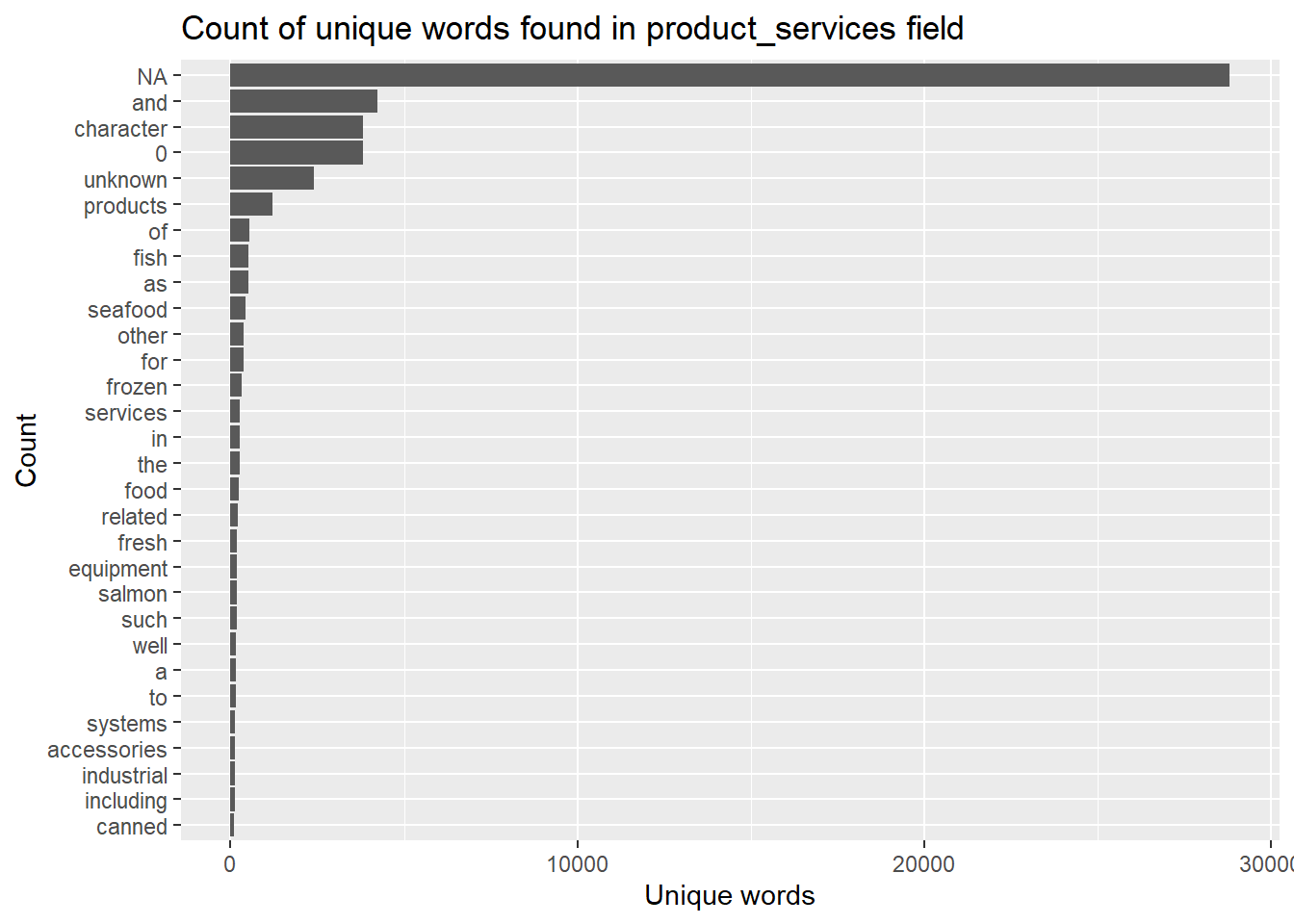

Observations

The bar chart reveals that the unique words contains some words that may not be useful to use. For instance “a” and “to”. In the word of text mining we call those words stop words. We will remove these words from the analysis as they are fillers used to compose a sentence.

In addition, there is also a high number of the words NA, character, 0, unknown, products which are not representative of the products_services field. Hence, we will add them into the stop_words dataset in tidytext so that they can be filtered out.

3.3.1. Adding stop words into the tidytext stop_words dataset

We will first retrieve the list of stop_words dataset. Next, we will create a list additional_stop_words, that will contains the additional words that we want to remove.

We will then use bind_rows() to add the additional_stop_words into the stop_words dataset. We will call distinct() function to make sure that there is no duplicate stop_words in the dataset.

Code

# Retrieve the current stop_words dataset
data(stop_words)

# Create a vector containing the additional stop words
additional_stop_words <- c(NA_character_, "character", "0", 
                           "unknown", "products")

# Add the additional stop words to the stop_words dataset and remove any duplicate entries
stop_words <- bind_rows(stop_words, 
                        tibble(word = additional_stop_words))

stop_words <- distinct(stop_words)

3.3.2. Removing the Stop Words

Code

nodes_combined_no_stopwords <- nodes_combined_unnest %>%
  anti_join(stop_words)

We can then visualise the words after removing the stop words.

Code

nodes_combined_no_stopwords %>%
  count(word, sort = TRUE) %>%
  top_n(30) %>%
  mutate(word = reorder(word, n)) %>%
  ggplot(aes(x = word, y = n)) +
  geom_col() +
  xlab(NULL) +
  coord_flip() +
      labs(x = "Count",
      y = "Unique words",
      title = "Count of unique words found in product_services field")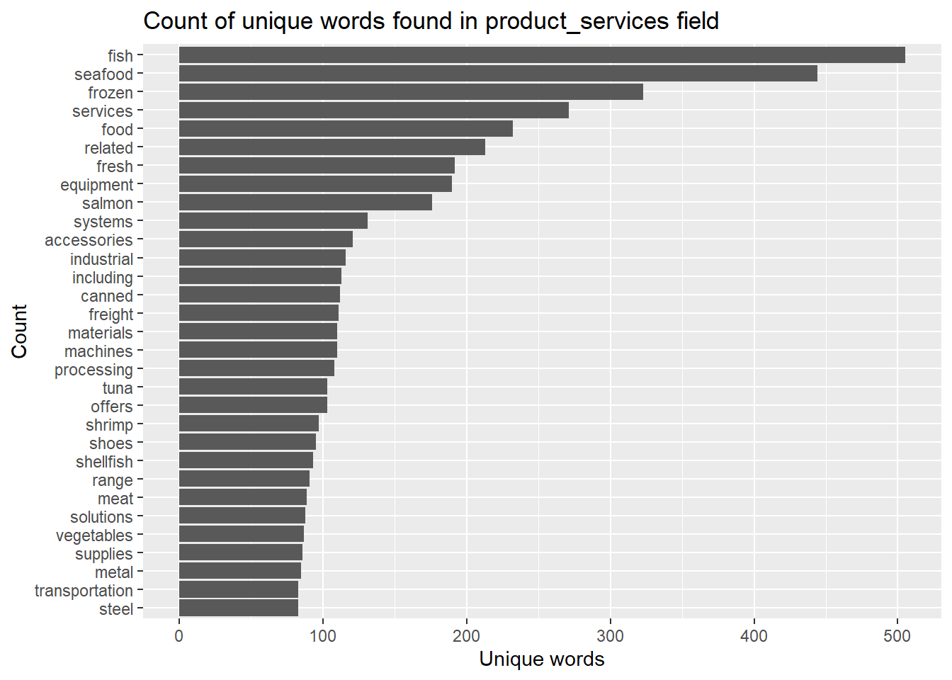

3.3.3. Retrieving the nodes that contain fishing-related keywords

In order to find the companies that are related to fishing, we will extract all the nodes that contain fishing-related keywords.

Code

# build the fishing-related nodes
nodes_fishing <- nodes_combined_no_stopwords %>%
  filter(word %in% c("fish", "fishing", "seafood", "seafoods", "salmon",
                     "shrimp", "prawn", "crabs", "squid", "oysters",
                     "clams", "trout", "cod", "lobster", "catfish", 
                     "mackerel", "herring", "pollock", "tuna", 
                     "trout", "finfish", "tilapias", "caviar")) %>%
  select(id, label, country, type, revenue_omu, word) %>%
  group_by(id, label, country, type, revenue_omu, word) %>%
  arrange(label) %>%
  ungroup()


# Combine the words for the same id using aggregate(), so that we will end up with 1 record per node
nodes_fishing_prod <- nodes_fishing %>%
  group_by(id) %>%
  summarize(product_services = paste(unique(word), collapse = ","),
            label = unique(label), country = unique(country), 
            type = unique(type), revenue_omu = unique(revenue_omu),
            .groups = "drop") %>%
  select(label, country, type, revenue_omu, product_services) %>%
  rename(id = label)

# build the edges table based on the nodes in nodes_combined_fishing
edges_fishing <- final_mc3_edges %>%
  filter(source %in% nodes_fishing_prod$id |
         target %in% nodes_fishing_prod$id)  

Code

nodes_fishing_prod <- nodes_fishing_prod %>%
  rename(label = id) %>%
  mutate(id=row_number())

edges_fishing <- edges_fishing %>%
  rename(from = source) %>%
  rename(to = target)

4. Data Exploration & Visualisation

4.1. Understanding the Fishing-related Companies - Country

For this section, we will find out more about the fishing-related companies, particularly on the country that they belong.

Code

# Computing the count of companies by country
nodes_fishing_prod_ctry <- nodes_fishing_prod %>%
  group_by(country) %>%
  summarize(ctry_cnt = n())

ggplot_tm <- ggplot(nodes_fishing_prod_ctry, 
       aes(area = ctry_cnt, label = country, fill = country)) +
  geom_treemap() +
  geom_treemap_text(aes(label = paste(country, "\nCount:", ctry_cnt)),
                    size = 10, hjust = 0.5, vjust = 0.5) +
  labs(title = "Countries of the fishing-related Companies") +
  theme_minimal() +
  theme(plot.title = element_text(hjust = 0.5))

ggplot_tm

Observations

From the treemap above, it was revealed that more than 50% of the fishing-related companies (383 out of 680 companies) are from Marebak, Oceanus, ZH and Nalakond. Most of the unlabeled grids at the top right hand corner of the plot are countries with 1 company that is involved in fishing-related products and services.

4.2. Understanding the Fishing-related Companies - revenue_omu

Code

# Computing the count of companies by country
nodes_fishing_prod_ctry <- nodes_fishing_prod %>%
  group_by(country) %>%
  summarize(ctry_cnt = n(), across(everything())) %>%
  ungroup()

treemap(nodes_fishing_prod_ctry,
        index=c("country", "label"),
        vSize="revenue_omu",
        vColor="revenue_omu",
        title="Fishing-related Companies by Revenue_omu and Country",
        title.legend = "country",
        position.legend = "right"
        )

Observations

If we were to look from the perspective of revenue_omu, From the revenue_omu treemap above, it is interesting to notice that the bigger revenue earners are from ZH, Rio Isla and Oceanus.

It was noted that there are 6 domineering companies in ZH which have the highest revenues. These companies were not highlighted in any of the earlier analysis. We will investigate further into Morgan Group, the highest revenue earner, in attempt to identify anomalies.

4.2.1. Looking into the Highest Revenue Earner - Morgan Group

From the observation in Section 4.2, it was revealed that Morgan Group, from ZH, has the highest revenue_omu, but was not surfaced in any of the earlier analysis. Hence, we will probe a little further into this company, looking at the products_services, beneficial owner and company contacts.

Code

morgan <-  mc3_nodes_raw %>%
  filter(id == "Morgan Group") %>%
  mutate(revenue_omu = round(revenue_omu, 2)) %>%
  select(id, country, type, revenue_omu, product_services)

# Including the commas for easy readability
morgan$revenue_omu <- scales::comma(morgan$revenue_omu, accuracy = 0.01)

datatable(morgan,
          class="stripe",
          caption = "\nTable 6: Information about 'Morgan Group' \n",
          colnames = c("Entity", "Country", "Type", "Revenue_omu",
                       "Products & Services"),
          options = list(columnDefs = list(list(className = 'dt-center',
                                                targets="_all"))))

Code

# Getting information from the original edge file
morgan_edges <- mc3_edges_raw %>%
  filter(source == "Morgan Group" | target == "Morgan Group")

datatable(morgan_edges,
          class="stripe",
          caption = "\nTable 7: Information about 'Morgan Group' \n",
          colnames = c("Source", "Target", "Type", "Weights"),
          options = list(columnDefs = list(list(className = 'dt-center',
                                                targets="_all"))))

Observations

From the original records, we have very limited information about Morgan Group and its sole Beneficial Owner, Jason Cole. We observed that Morgan Group as a Company, only has a revenue_omu value of 10,385.72. From the records, we do not have any information of any subsidiary companies where Morgan Group is a Beneficial Owner, even though the revenue_omu is extremely high.

In addition, Jason Cole is not an Beneficial Owner of other Companies within the network. Hence, we could not determine whether the company is involved in any suspicious activities.

In view of the high revenue_omu of Morgan Group, as a Beneficial Owner, it was suggested that we put Morgan Group under watchlist for anomalies, until there are additional information about the company or its beneficial owner.

4.3. Investigating on the Companies Identified Earlier

In this section, we will cross-reference back to the list of Companies that were being identified in Section 3.1.2.1, to find if there is any anomalies.

Code

nodes_fishing_prod_int_coy <- nodes_fishing_prod %>%
  filter(label %in% coy_bo_above_50$source |
           label %in% coy_cc_above_5$source) %>%
  distinct()

edge_fishing_int_coy <- edges_fishing %>%
  filter(from %in% nodes_fishing_prod_int_coy$label)

Code

# build the variables to plot nw
id1_int_coy <- edge_fishing_int_coy %>%
  select(from) %>%
  rename(id = from)

id2_int_coy <- edge_fishing_int_coy %>%
  select(to) %>%
  rename(id = to)

# create a new nodes data table derived from the source and target of edge data. This would ensure that only nodes with connections will be included.
fish_nodes_combined_int_coy <- rbind(id1_int_coy, id2_int_coy) %>%
  distinct()

fish_nodes_combined_int_coy <- fish_nodes_combined_int_coy %>%
  mutate( group = case_when(
    id %in% edge_fishing_int_coy$from ~ "Company",
    id %in% edge_fishing_int_coy$to & 
      edge_fishing_int_coy$type == "Beneficial Owner" ~ "Beneficial Owner",
    id %in% edge_fishing_int_coy$to & 
      edge_fishing_int_coy$type == "Company Contacts" ~ "Company Contacts"
    )
  ) %>%
  arrange(id) 

Code

visNetwork(fish_nodes_combined_int_coy,
           edge_fishing_int_coy,
           main = "Network Graph of Fishing-related Companies with High Number of Beneficial Owners or Company Contacts") %>%
  visIgraphLayout(layout = "layout_with_fr") %>%
  visLayout(randomSeed = 1234) %>%
  visOptions(highlightNearest = list(enabled = T, degree = 2, hover = T),
             nodesIdSelection = TRUE) %>%
  visNodes(id = fish_nodes_combined_int_coy$id, size=50) %>%
  visLegend(width = 0.1, position = "right", main = "Group") %>%
  visEdges(smooth = list(enabled = TRUE, type = "curvedCW"))

Observation

From the network graph above, it is observed that both Aqua Aura SE Marine life and Congo Rapids Ltd. Corporation have significantly more Beneficial Owners and Company Contacts compared to the other two.

With the above observations, we will extract out the information on the above-mentioned companies to take a look at their other available information (i.e. country, revenue_omu and products_services) from both the dataset that contains fishing-related nodes and the original raw dataset.

Company Information From Fishing-related List

We will extract the respective companies’ information from the fishing-related dataset (nodes_fishing_prod) to particularly look at the list of product & services that these companies are involved in and their respective revenue_omu. However, we are mindful that some of these information were not available (i.e. NA) and hence we will have to discard these records from the analysis.

First of all, we will extract the companies that we want by using filter(). We will then compute the total_revenue and including it as an additional column to the nodes_fishing_prod_int_coy_nw_df dataframe.

Design Consideration

1. A horizontal bar chart is used, with the y-axis showing the company names so that it can be easily read.
2. The results are sorted from the highest total revenue of the company to the lowest.
3. Different colours were used to differentiate the companies.
4. As it is possible that there are multiple records for one company (due to different country, revenue_omu and products_services), the bars for each company are stacked up, with stacked segment representing the different variance of the company, with its country and revenue_omu will also be shown on the graph.
5. Additional information of the company such as the country, revenue_omu and total_revenue are included as part of the tooltip, when the mouse hovers to the respective bars.
6. Information on the product_services will not be included as part of the tooltip, as the data is too lengthy and might be difficult to read. Instead, the information will be included in the datatable below the plot.
7. For easier readability, included thousand separators (commas) and rounded to 2 decimal places for revenue_omu and total_revenue.
8. Lastly, as the datatable is showing all the information of the companies, it was deemed unsuitable to be placed beside the plot.

Code

nodes_fishing_prod_int_coy_nw_df <- nodes_fishing_prod %>%
  filter(label %in% fish_nodes_combined_int_coy$id) %>%
  group_by(label) %>%
  distinct() %>%
  summarise(total_revenue = sum(revenue_omu), across(everything())) %>%
  mutate(revenue_omu = round(revenue_omu, 2)) %>%
  mutate(total_revenue = round(total_revenue, 2)) %>%  
  select(label, country, revenue_omu, total_revenue, product_services) 

# plotting the graph
plot_fish <- ggplot(nodes_fishing_prod_int_coy_nw_df, 
               aes(x = reorder(label, total_revenue), 
                   y = revenue_omu, fill = label,
                   text = paste("Company: ", label, 
                                "<br>Country: ", country,
                                "<br>Individual Revenue by Entity: ", 
                                revenue_omu,
                                "<br>Total Revenue: ", total_revenue))) +
  geom_bar(stat = "identity") +
  coord_flip() +
  labs(x = "Company", y = "Total Revenue", 
       title = "Company of Interest - Total Revenue") +
  ylim(0, 55000) +
  scale_fill_brewer(palette = "Set3") +
  theme_minimal() +
  theme(axis.title.y = element_blank()) + 
  guides(fill = FALSE) 

plotly_plot <- ggplotly(plot_fish, tooltip = "text")
plotly_plot

Code

# Including the thousand separator (comma) for easy readability
nodes_fishing_prod_int_coy_nw_df$revenue_omu <-
  scales::comma(nodes_fishing_prod_int_coy_nw_df$revenue_omu, 
                accuracy = 0.01)

nodes_fishing_prod_int_coy_nw_df$total_revenue <-
  scales::comma(nodes_fishing_prod_int_coy_nw_df$total_revenue, 
                accuracy = 0.01)

# Showing the datatable
datatable(nodes_fishing_prod_int_coy_nw_df,
          class="stripe",
          caption = "\nTable 8: Company Information From Fishing-related List\n",
          colnames = c("Company", "Country", "Revenue_omu", "Total Revenue",
                       "Products & Services"),
          options = list(columnDefs = list(list(className = 'dt-center',
                                                targets="_all"))))

Company Information From Original Raw DataSet

We will extract the respective companies’ information from the orginal raw dataset (mc3_nodes_raw) to particularly look at the list of product & services that these companies are involved in and their respective revenue_omu. However, we are mindful that some of these information were not available (i.e. NA) and hence we will have to discard these records from the analysis.

First of all, we will extract the companies that we want by using filter(). We will then compute the total_revenue and including it as an additional column to the int_coy_raw dataframe.

Design Consideration

1. A horizontal bar chart is used, with the y-axis showing the company names so that it can be easily read.
2. The results are sorted from the highest total revenue of the company to the lowest.
3. Different colours were used to differentiate the companies.
4. As it is possible that there are multiple records for one company (due to different country, revenue_omu and products_services), the bars for each company are stacked up, with stacked segment representing the different variance of the company, with its country and revenue_omu will also be shown on the graph.
5. Additional information of the company such as the country, revenue_omu and total_revenue are included as part of the tooltip, when the mouse hovers to the respective bars.
6. Information on the product_services will not be included as part of the tooltip, as the data is too lengthy and might be difficult to read. Instead, the information will be included in the datatable below the plot.
7. For easier readability, included thousand separators (commas) and rounded to 2 decimal places for revenue_omu and total_revenue.
8. Lastly, as the datatable is showing all the information of the companies, it was deemed unsuitable to be placed beside the plot.

Code

# Preparing the data for plotting and presenting as a datatable
int_coy_raw <- mc3_nodes_raw %>%
  filter(id %in% fish_nodes_combined_int_coy$id) %>%
  group_by(id) %>%
  distinct()

# Preparing the data for plotting and presenting as a datatable
int_coy_raw <- int_coy_raw[complete.cases(int_coy_raw), ] %>%
  summarise(total_revenue = sum(revenue_omu), across(everything())) %>%
  mutate(revenue_omu = round(revenue_omu, 2)) %>%
  mutate(total_revenue = round(total_revenue, 2)) %>%
  select(id, country, type, revenue_omu, total_revenue, product_services)

# plotting the graph
plot_raw <- ggplot(int_coy_raw, aes(x = reorder(id, total_revenue), 
                               y = revenue_omu, fill = id,
                               text = paste("Company: ", id, 
                                            "<br>Country: ", country,
                                            "<br>Individual Revenue by Entity: ",
                                            revenue_omu,
                                            "<br>Total Revenue: ", total_revenue))) +
  geom_bar(stat = "identity") +
  coord_flip() +
  labs(x = "Company", y = "Total Revenue", 
       title = "Company of Interest - Total Revenue (from Raw Dataset)") +
  ylim(0, 160000) +
  scale_fill_brewer(palette = "Set3") +
  theme_minimal() +
  theme(axis.title.y = element_blank()) + 
  guides(fill = FALSE) 

plotly_plot <- ggplotly(plot_raw, tooltip = "text")
plotly_plot

Code

# Including the thousand separator (comma) for easy readability
int_coy_raw$revenue_omu <- 
  scales::comma(int_coy_raw$revenue_omu, accuracy = 0.01)

int_coy_raw$total_revenue <- 
  scales::comma(int_coy_raw$total_revenue, accuracy = 0.01)

# Presenting the datatable with the detailed information of each company  
datatable(int_coy_raw, class="stripe",
          caption = "\nTable 9: Company Information From Fishing-related List (RAW)\n",
          colnames = c("Company", "Country", "Type", "Revenue_omu", "Total Revenue",
                       "Products & Services"),
          options = list(columnDefs = list(list(className = 'dt-center',
                                                           targets="_all"))))

Observation

Aqua Aura SE Marine life

From the analysis of the data extracted from Fishing-related products and services, Aqua Aura SE Marine life actually has 3 different records, with 2 under the country Rio Isla and the other is under Oceanus.

When we compared the results of Aqua Aura SE Marine life with the raw dataset, it was noted that they also have smaller business footprints in other countries such as Icarnia, Nalakond and Coralmarica; as well as two other records under Oceanus. However, as we do not have any information on the products and services that they were involved, we were unable to determine whether it is involved in any suspicious illegal fishing activities.

Reference to Section 3.1.2.1 - Visualisation of the Relationship of Company to Individual

In terms of Beneficial Owners, it was revealed that Dale Rhodes and Cynthia Murphy are also Beneficial Owners to Irish Mackerel S.A. de C.V. Marine biology, which is not related to fishing, based on the original dataset.

With the above information, it is suggested to put Aqua Aura SE Marine life under watchlist for anomalies, until there are additional information about the company and/or its beneficial owners and company contacts.

Congo Rapids Ltd. Corporation

From the fishing-related products and services dataset, Congo Rapids Ltd. Corporation only deals with salmon. When we compared this with the results extracted from the raw dataset, it was observed that Congo Rapids Ltd. Corporation only provides products related to children’s accessories (stationery), which contributed to its main revenue.

Reference to Section 3.1.2.1 - Visualisation of the Relationship of Company to Individual We also observed that Congo Rapids Ltd. Corporation has multiple beneficial owners, and one of them, Jeremy Lee, is also a beneficial owner of Niger Bend AS Express, which was listed as a Cruise ship holidays company. Unfortunately, we do not have any other information about Jeremy Lee and hence we could not determine whether the 2 companies nor Jeremy Lee are involved in any suspicious illegal fishing activities.

However, it is worth mentioning to note that Congo Rapids Ltd. Corporation is from the country Brindivaria, which is not one of the more common countries for companies with fishing-related businesses.

From the above information gathered, it is suggested to put Congo Rapids Ltd. Corporation, Niger Bend AS Express and Jeremy Lee under watchlist for anomalies, until there are additional information about them.

5. Conclusion

Even though we could not confidently identify anomalies from the analysis, we would suggest including the following business groups into a watchlist for further monitoring, until there is additional information about them:

• Morgan Group and Jason Cole (From Section 4.2: due to extremely high revenue_omu in a sole Beneficial Owner Company, with no other sub-businesses found in the records).
• Aqua Aura SE Marine life (From Section 4.3: Company has business footprints in multiple countries, significantly large number of Beneficial Owners and Company Contacts).
• Congo Rapids Ltd. Corporation, Niger Bend AS Express and Jeremy Lee (From Section 4.3: Congo is not from one of the more common countries and its primary source revenue is not related to fishing).

Data Quality Issues

There were also a number of data quality issues, such data inconsistency and unclean data that hindered the data analysis.

Node Records

• Missing values (NA), unknown and character(0) in revenue_omu and product_services fields.
• Not all records are fishing-related.
• Large number of Beneficial Owners and Company Contacts could not be found here, even though they were present in the Edge records.

Edges Records

• source field containing sub-lists.
• target field containing salutations of some individuals.
• Records found here could not be found in Nodes Records.