Code
pacman::p_load(ggstatsplot, tidyverse, rstantools)In this exercise using Exam_data, we will be using ggstatsplot and tidyverse. rstantools and PMCMRplus are also be required for plotting the ONEWAY ANOVA graph.
pacman::p_load(ggstatsplot, tidyverse, rstantools)For this exercise, Exam_data.csv provided will be imported into R by using read_csv() of readr package.
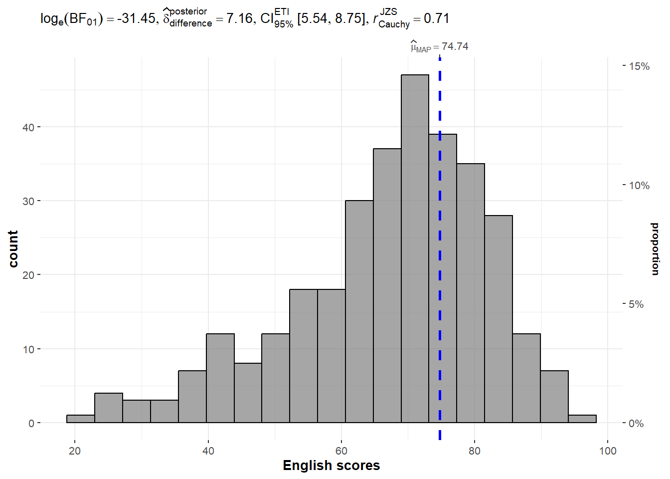
exam_data <- read_csv("data/Exam_data.csv")gghistostats() methodIn the code chunk below, gghistostats() is used to to build an visual of one-sample test on English scores, with default information: - statistical details - Bayes Factor - sample sizes - distribution summary.
set.seed(1234)

gghistostats(
  data = exam_data,
  x = ENGLISH,
  type = "bayes",
  test.value = 60,
  xlab = "English scores"
)
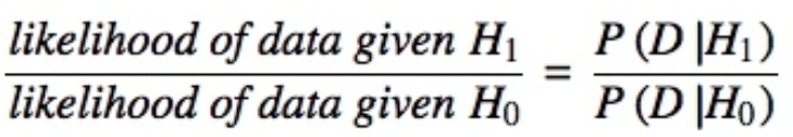
A Bayes factor is the ratio of the likelihood of one particular hypothesis to the likelihood of another. It can be interpreted as a measure of the strength of evidence in favor of one theory among two competing theories.
That’s because the Bayes factor gives us a way to evaluate the data in favor of a null hypothesis, and to use external information to do so. It tells us what the weight of the evidence is in favor of a given hypothesis.
When we are comparing two hypotheses, H1 (the alternate hypothesis) and H0 (the null hypothesis), the Bayes Factor is often written as B10. It can be defined mathematically as
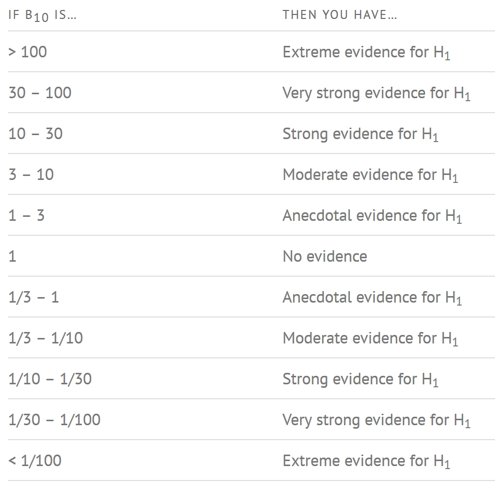
A Bayes Factor can be any positive number. One of the most common interpretations is this one—first proposed by Harold Jeffereys (1961) and slightly modified by Lee and Wagenmakers in 2013:
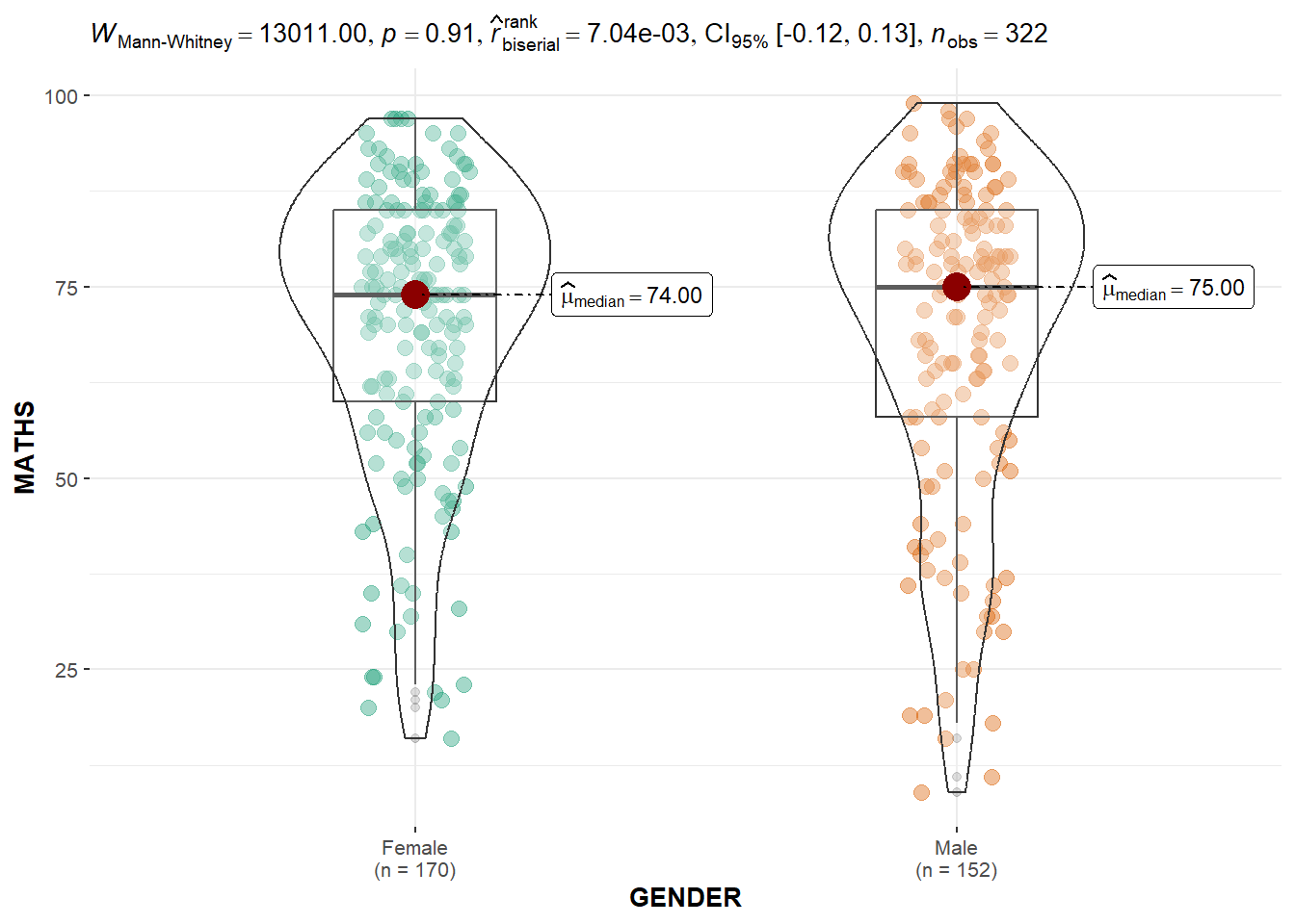
ggbetweenstats() methodThe code chunk below shows ggbetweenstats() being used to build a visual for two-sample mean test of Maths scores by gender.Default information: - statistical details - Bayes Factor - sample sizes - distribution summary
ggbetweenstats(
  data = exam_data,
  x = GENDER,
  y = MATHS,
  type = "np",
  messages = FALSE
)
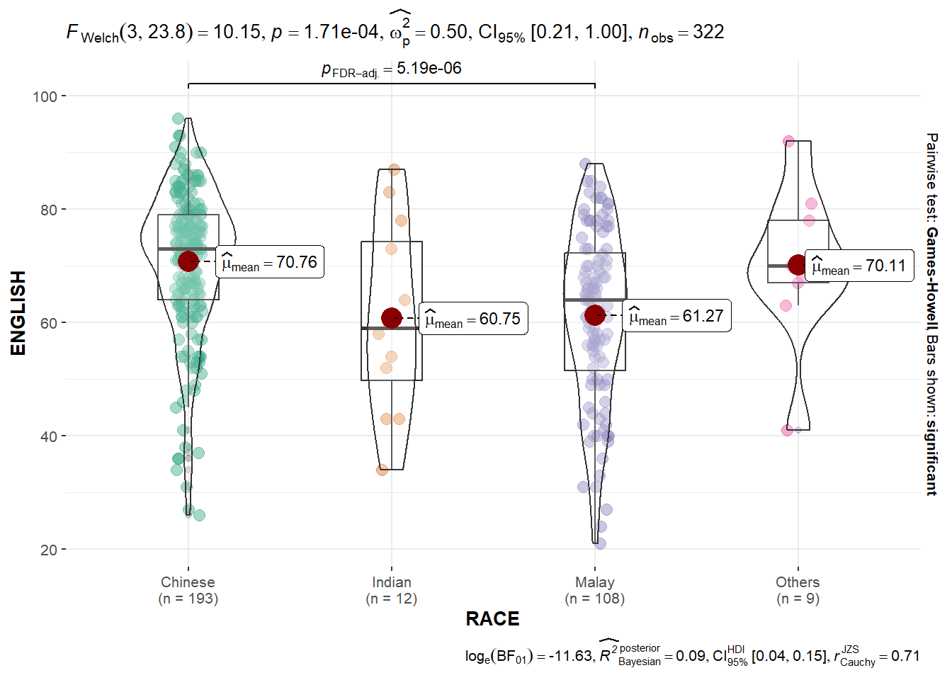
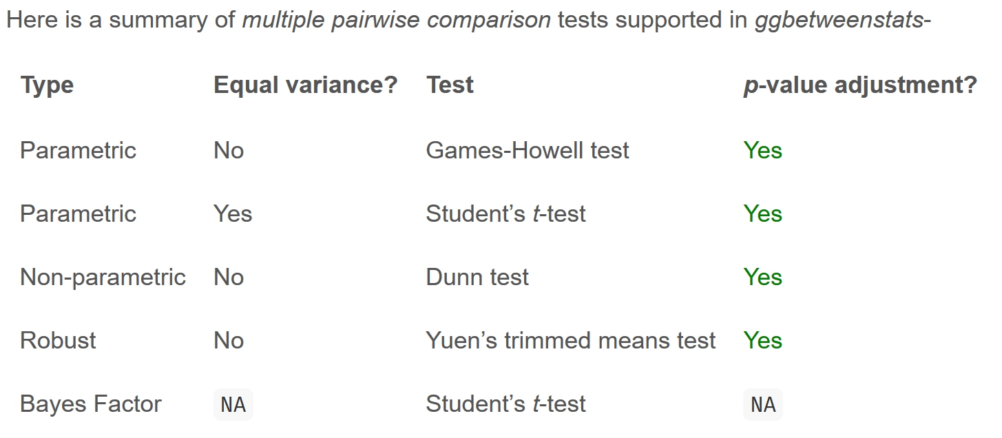
ggbetweenstats() methodThe code chunk below shows ggbetweenstats() being used to build a visual for One-way ANOVA test on English score by race.
ggbetweenstats(
  data = exam_data,
  x = RACE,
  y = ENGLISH,
  type = "p",
  mean.ci = TRUE,
  pairwise.comparisons = TRUE,
  pairwise.display = "s",
  p.adjust.method = "fdr",
  messages = FALSE
)
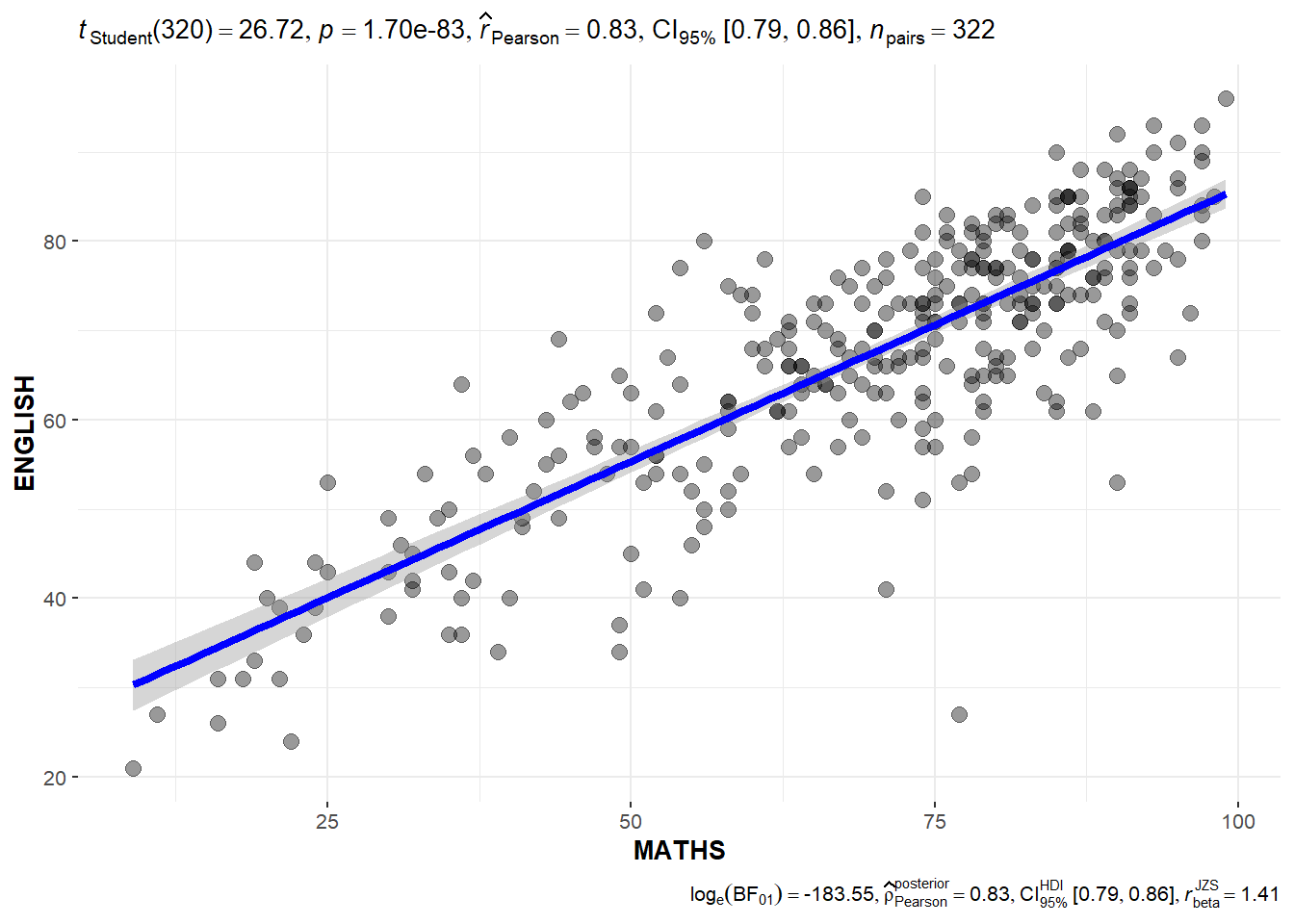
ggscatterstats() methodThe code chunk below shows ggscatterstats() being used to build a visual for Significant Test of Correlation between Maths scores and English scores.
ggscatterstats(
  data = exam_data,
  x = MATHS,
  y = ENGLISH,
  marginal = FALSE,
  )
ggbarstats() methodsIn the code chunk below, the Maths scores is binned into a 4-class variable by using cut().
exam1 <- exam_data %>%
  mutate(MATHS_bins =
           cut(MATHS,
               breaks = c(0,60,75,85,100))
)
We then use ggbarstats() to build a visual for Significant Test of Association, as shown in the code chunk below.
ggbarstats(exam1,
           x = MATHS_bins,
           y = GENDER)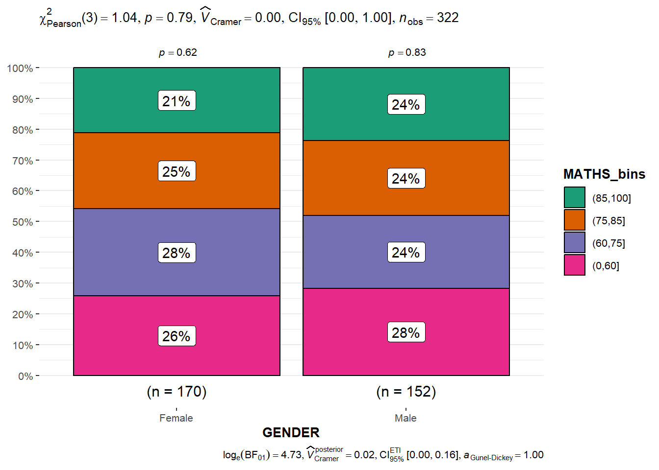
In this section, we will visualise model diagnostic and model parameters by using parameters package.
Toyota Corolla case study will be used. The purpose of study is to build a model to discover factors affecting prices of used-cars by taking into consideration a set of explanatory variables.
pacman::p_load(readxl, performance, parameters, see)For this exercise, ToyotaCorolla.xls provided will be imported into R by using read_xls() of readxl package.
car_resale <- read_xls("data/ToyotaCorolla.xls",
                       "data")
car_resale
# A tibble: 1,436 × 38
Id Model Price Age_08_04 Mfg_Month Mfg_Year KM Quarterly_Tax Weight
<dbl> <chr> <dbl> <dbl> <dbl> <dbl> <dbl> <dbl> <dbl>
1 81 TOYOTA … 18950 25 8 2002 20019 100 1180
2 1 TOYOTA … 13500 23 10 2002 46986 210 1165
3 2 TOYOTA … 13750 23 10 2002 72937 210 1165
4 3 TOYOTA… 13950 24 9 2002 41711 210 1165
5 4 TOYOTA … 14950 26 7 2002 48000 210 1165
6 5 TOYOTA … 13750 30 3 2002 38500 210 1170
7 6 TOYOTA … 12950 32 1 2002 61000 210 1170
8 7 TOYOTA… 16900 27 6 2002 94612 210 1245
9 8 TOYOTA … 18600 30 3 2002 75889 210 1245
10 44 TOYOTA … 16950 27 6 2002 110404 234 1255
# ℹ 1,426 more rows
# ℹ 29 more variables: Guarantee_Period <dbl>, HP_Bin <chr>, CC_bin <chr>,
# Doors <dbl>, Gears <dbl>, Cylinders <dbl>, Fuel_Type <chr>, Color <chr>,
# Met_Color <dbl>, Automatic <dbl>, Mfr_Guarantee <dbl>,
# BOVAG_Guarantee <dbl>, ABS <dbl>, Airbag_1 <dbl>, Airbag_2 <dbl>,
# Airco <dbl>, Automatic_airco <dbl>, Boardcomputer <dbl>, CD_Player <dbl>,
# Central_Lock <dbl>, Powered_Windows <dbl>, Power_Steering <dbl>, …lm()The code chunk below is used to calibrate a multiple linear regression model by using lm() of Base Stats of R.
model <- lm(Price ~ Age_08_04 + Mfg_Year + KM +
              Weight + Guarantee_Period, data = car_resale)
model
Call:
lm(formula = Price ~ Age_08_04 + Mfg_Year + KM + Weight + Guarantee_Period,
    data = car_resale)

Coefficients:
     (Intercept)         Age_08_04          Mfg_Year                KM
      -2.637e+06        -1.409e+01         1.315e+03        -2.323e-02
          Weight  Guarantee_Period
1.903e+01 2.770e+01 Using check_collinearity() method from the performance package
check_collinearity(model)# Check for Multicollinearity
Low Correlation
Term VIF VIF 95% CI Increased SE Tolerance Tolerance 95% CI
KM 1.46 [ 1.37, 1.57] 1.21 0.68 [0.64, 0.73]
Weight 1.41 [ 1.32, 1.51] 1.19 0.71 [0.66, 0.76]
Guarantee_Period 1.04 [ 1.01, 1.17] 1.02 0.97 [0.86, 0.99]
High Correlation
Term VIF VIF 95% CI Increased SE Tolerance Tolerance 95% CI
Age_08_04 31.07 [28.08, 34.38] 5.57 0.03 [0.03, 0.04]
Mfg_Year 31.16 [28.16, 34.48] 5.58 0.03 [0.03, 0.04]check_c <- check_collinearity(model)
plot(check_c)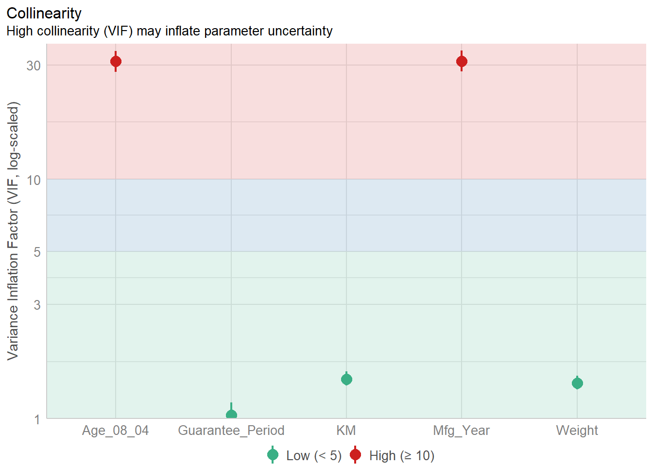
Using check_normality() method from the performance package
model1 <- lm(Price ~ Age_08_04 + KM +
              Weight + Guarantee_Period, data = car_resale)

check_n <- check_normality(model1)

plot(check_n)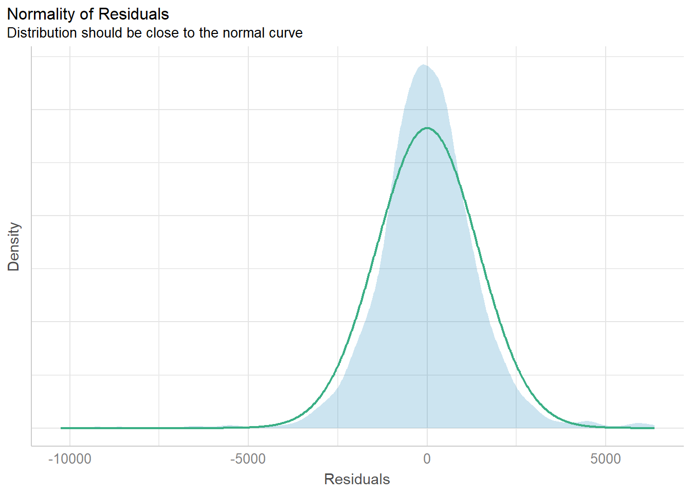
Using check_heteroscedasticity() method from the performance package
check_h <- check_heteroscedasticity(model1)

plot(check_h)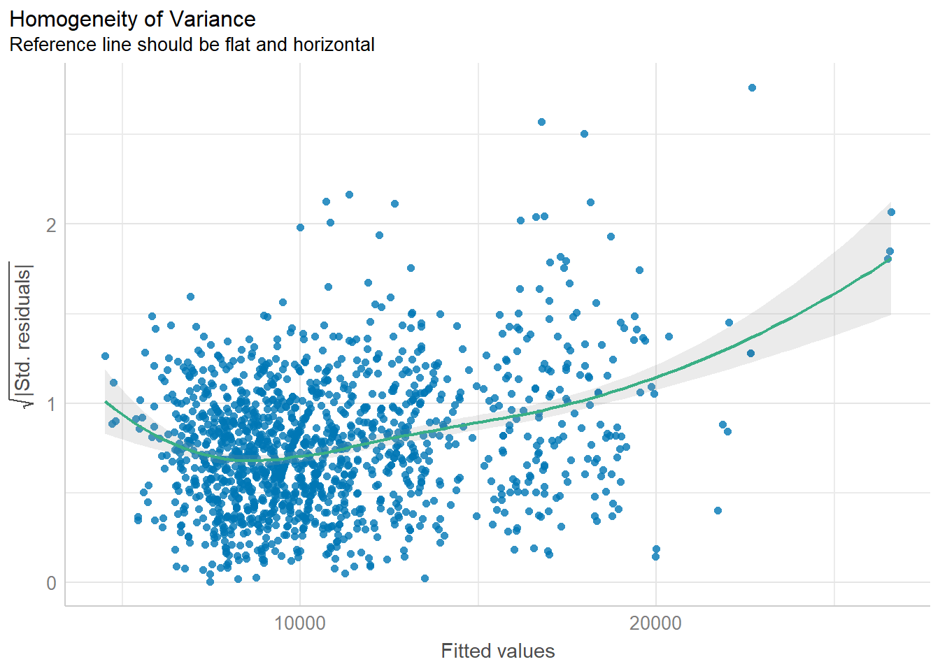
We can also perform the complete by using check_model().
check_model(model1)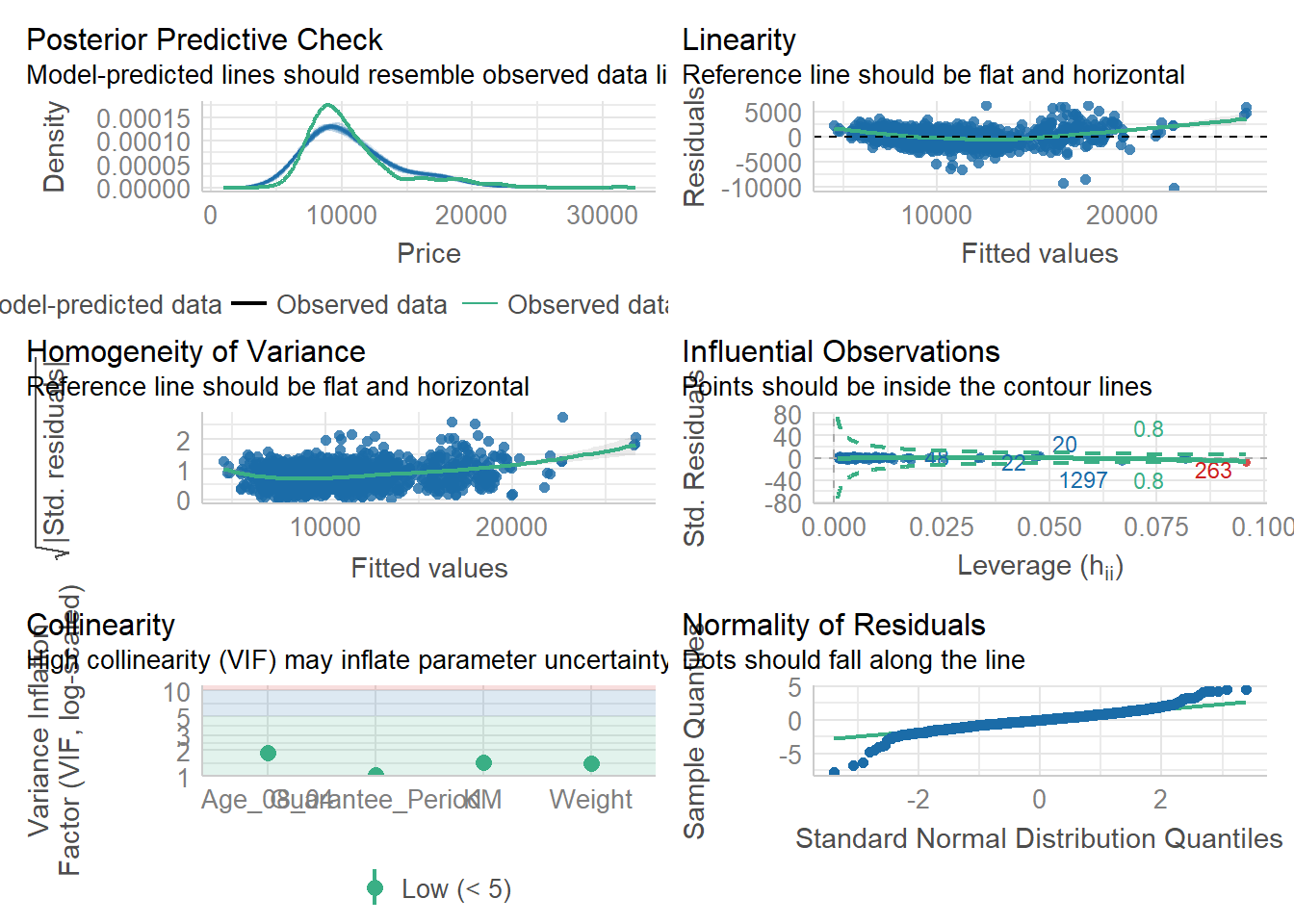
In the code below, plot() of see package and parameters() of parameters package are used to visualise the parameters of a regression model.
plot(parameters(model1))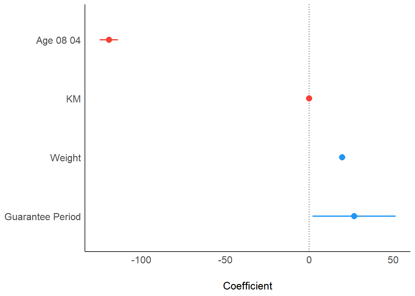
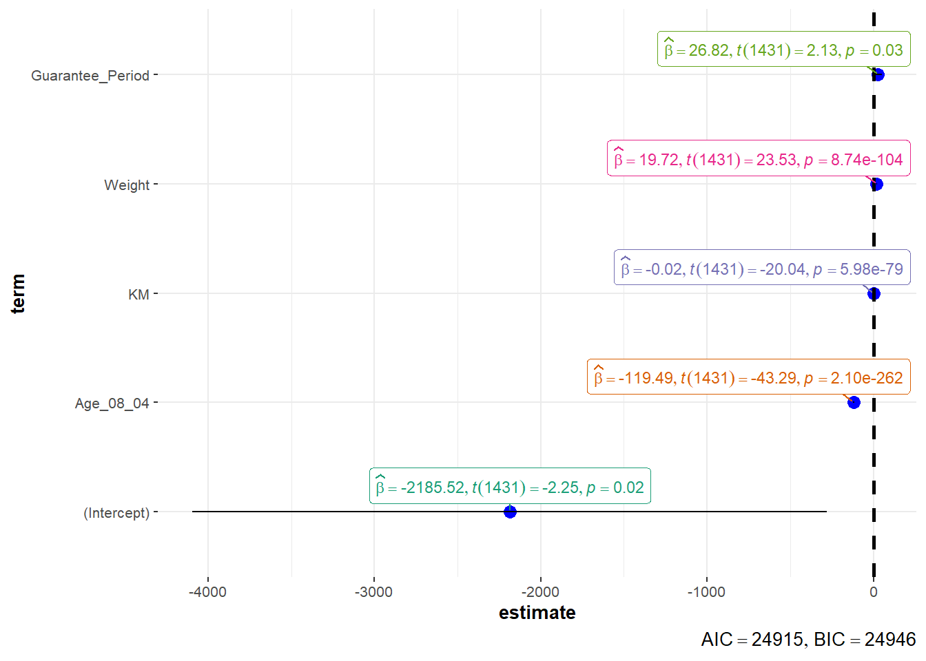
ggcoefstats() methodThis example uses ggcoefstats() of ggstatsplot package to visualise the parameters of a regression model.
ggcoefstats(model1,
            output = "plot")