Show the codes
pacman::p_load(jsonlite, tidygraph, ggraph, visNetwork, lubridate,
igraph, tidyverse, DT)With reference to the Mini-Challenge 2 of VAST Challenge 2023 and by using appropriate static and interactive statistical graphics methods, we will help FishEye identify companies that may be engaged in Illegal, unreported, and unregulated (IUU) fishing.
Use visual analytics to identify temporal patterns for individual entities and between entities in the knowledge graph FishEye created from trade records. Categorize the types of business relationship patterns you find.
For this task, we will make use of the mc2_challenge_graph.json provided for the data analysis and visualisation.
The required R library packages are being loaded. For this exercise, we will make use of the following R library packages.
The code chunk below uses pacman::p_load() to check if the above packages are installed. If they are, they will be loaded into the R environment.
pacman::p_load(jsonlite, tidygraph, ggraph, visNetwork, lubridate,
igraph, tidyverse, DT)We will first load each of the data files into the environment and perform data wrangling.
Based on the VAST 2023 data notes, column dataset will always be ‘mc2’, to represent this set of data belongs to mini challenge 2. As such, we will not import this column into the R environment.
We will first load in the main file, mc2_challenge_graph.json, then extract the nodes and edges (links) information out.
mc2 <- fromJSON("data/mc2_challenge_graph.json")mc2_nodes <- as_tibble(mc2$nodes) %>%
select(id, shpcountry, rcvcountry)mc2_edges <- as_tibble(mc2$links) %>%
select(source, target, arrivaldate, hscode,
weightkg, valueofgoods_omu, volumeteu,
valueofgoodsusd)glimpse() of dyplr.glimpse(mc2_nodes)Rows: 34,576
Columns: 3
$ id <chr> "AquaDelight Inc and Son's", "BaringoAmerica Marine Ges.m.b…
$ shpcountry <chr> "Polarinda", NA, "Oceanus", NA, "Oceanus", "Kondanovia", NA…
$ rcvcountry <chr> "Oceanus", NA, "Oceanus", NA, "Oceanus", "Utoporiana", NA, …glimpse(mc2_edges)Rows: 5,464,378
Columns: 8
$ source <chr> "AquaDelight Inc and Son's", "AquaDelight Inc and Son…
$ target <chr> "BaringoAmerica Marine Ges.m.b.H.", "BaringoAmerica M…
$ arrivaldate <chr> "2034-02-12", "2034-03-13", "2028-02-07", "2028-02-23…
$ hscode <chr> "630630", "630630", "470710", "470710", "470710", "47…
$ weightkg <int> 4780, 6125, 10855, 11250, 11165, 11290, 9000, 19490, …
$ valueofgoods_omu <dbl> 141015, 141015, NA, NA, NA, NA, NA, NA, NA, NA, NA, N…
$ volumeteu <dbl> 0, 0, 0, 0, 0, 0, 0, 0, 0, 0, 0, 0, 0, 0, 0, 0, 0, 0,…
$ valueofgoodsusd <dbl> NA, NA, NA, NA, NA, NA, 87110, 188140, NA, 221110, 58…There are a number of chr data type columns in both mc2_nodes and mc2_edges, as a good practice, we will trim away any possible leading and trailing white spaces of the data, before we perform any analysis.
The arrivaldate has the format of ‘YYYY-MM-DD’ and is treated as chr data type instead of date data type.
A closer examination on the columns valueofgoods_omu, volumeteu, valueofgoodsusd columns revealed that there are also a large number of NA (missing values) and are deemed as as incomplete. We will drop these columns from analysis.
We will also need to filter out any possible duplicate records by using the distinct() function.
Drop columns valueofgoods_omu, volumeteu and valueofgoodsusd since they are deemed as as incomplete for analysis.
Convert arrivaldate from chr data type to date data type by using ymd().
Extract the year component out from arrivaldate field with year().
Perform white space trimming for the chr columns,to remove any the leading and trailing white spaces with trimws().
Remove any possible duplicate records by using distinct()
Based on the data notes provided in the VAST Challenge, hscode refers to the Harmonized Commodity Description and Coding System Nomenclature (HS) developed by World Customs Organization (WCO). We will filter all the records based on the hscodes related to the context of the challenge. The relevant hscodes are prefixed with: 301, 302, 303, 304, 305, 306, 307, 308, 309, 1504, 1603, 1604, 1605 and 2301).
Aggregate the records, by deriving a weight column based on the number of records by grouping the source, target, hscode and year.
# For the edges data frame, we will make use of select() to extract
# and rearrange the columns.
mc2_edges <- mc2_edges %>%
  select(arrivaldate, source, target, hscode, weightkg) %>%
  mutate(arrivaldate = ymd(arrivaldate)) %>%
  mutate(year = year(arrivaldate)) %>%
  mutate(source = trimws(source)) %>%
  mutate(target = trimws(target)) %>%
  mutate(hscode = trimws(hscode)) %>%
distinct()# List of relevant hscodes related to fishing
rel_hscodes_3 <- c("301", "302", "303", "304", "305",
"306", "307", "308", "309")
rel_hscodes_4 <- c("1504", "1603", "1604", "1605", "2301")
# Extract the records with the above 1st 3 or 4 characters of hscodes
# using substr().
mc2_edges_aggregated <- mc2_edges %>%
filter((substr(hscode, 1, 3) %in% rel_hscodes_3) |
(substr(hscode, 1, 4) %in% rel_hscodes_4)) %>%
group_by(source, target, hscode, year) %>%
summarise(weight = n()) %>%
filter(source!=target) %>%
arrange(weight) %>%
ungroup()The nodes within the node file must be unique and since we have filtered and cleaned the data in mc2_edges_aggregated, we will make use of this to extract the nodes that are used here.
rbind() is used to combine the data in both source and target columns of mc2_edges_aggregated. We will then extract the unique records to form the nodes data frame.
id1 <- mc2_edges_aggregated %>%
  select(source) %>%
  rename(id = source)
id2 <- mc2_edges_aggregated %>%
  select(target) %>%
  rename(id = target)

# create a new nodes data table derived from the source and target of edge data. This would ensure that only nodes with connections will be included.

mc2_nodes_extracted <- rbind(id1, id2) %>%
distinct()# Build tbl_graph using the valid nodes and edges
mc2_graph <- tbl_graph(nodes = mc2_nodes_extracted,
edges = mc2_edges_aggregated,
directed = TRUE)As part of the data exploration and analysis, we will compute the centrality indices for the nodes and include them as attribute information to the nodes, before plotting them out for visualisation and analysis. We will also rename the id column to label and create a new column id by using the row_number() to ease the build of the visualisation graphs using visNetwork package.
Standard Binning were being performed on the computed centrality indices for the ease of analysis. The respective indices will be binned into 3 groups, Low, Medium and High.
We will also round up the centrality indices to 3 decimal points for the purpose of analysis.
# Renaming the id column to label and
# create a new column, id with the row_number()
mc2_graph <- mc2_graph %>%
  activate(nodes) %>%
  rename(label = id) %>%
mutate(id=row_number()) mc2_graph <- mc2_graph %>%
# Compute the degree centrality of each node and bin the scores into logical groups
mutate(degree_score = centrality_degree()) %>%
mutate(deg_bin = cut(degree_score, breaks = c(0, 200, 300, Inf),
labels = c("Low\n(0-199)",
"Medium\n(200-299)",
"High\n(>=300)\n"),
include.lowest = TRUE)) %>%
# Compute the closeness centrality and bin the scores into logical groups
mutate(closeness_score = round(centrality_closeness(), digits=3)) %>%
mutate(close_bin = cut(closeness_score,
breaks = c(0, 0.5, 0.8, Inf),
labels = c("Low\n(<=0.49)",
"Medium\n(0.5-0.79)",
"High\n(>=0.8)\n"),
include.lowest = TRUE)) %>%
# Compute the betweenness centrality and bin the scores into logical groups
mutate(betweenness_score = round(centrality_betweenness(), digits = 3)) %>%
mutate(bet_bin = cut(betweenness_score,
breaks = c(0, 50000, 100000, 500000, Inf),
labels = c("Low\n(0-49K)",
"Medium\n(50K-99K)",
"High\n(100K-499K)\n",
"Very High\n(>=500K)"),
include.lowest = TRUE))
# Computing the in-degree and out-degree centrality indices
# Convert to igraph for computing the in-degree and out-degree centrality
igraph_obj <- as.igraph(mc2_graph)
# In-degree centrality
in_degree_centrality <- degree(igraph_obj, mode = "in")
# Out-degree centrality
out_degree_centrality <- degree(igraph_obj, mode = "out")
# Eigenvector centrality
eigen_centrality <- eigen_centrality(igraph_obj, directed = TRUE)$vector
# Assigning in-degree and out-degree centrality as vertex attributes
V(mc2_graph)$in_degree <- in_degree_centrality
V(mc2_graph)$out_degree <- out_degree_centrality
V(mc2_graph)$eigen_score <- round(eigen_centrality, digits=3)
# Binning the in_degree scores and put as a variable inside mc2_graph
mc2_graph <- mc2_graph %>%
mutate(in_bin = cut(in_degree,
breaks = c(0, 300, 600, Inf),
labels = c("Low\n(<300)",
"Medium\n(300-599)",
"High\n(>=600)"),
include.lowest = TRUE)) %>%
# Binning the out_degree scores and put as a variable inside mc2_graph
mutate(out_bin = cut(out_degree,
breaks = c(0, 2, 300, 500, Inf),
labels = c("0-1", "Low\n(2-300)",
"Medium\n(301-500)",
"High\n(>500)"),
include.lowest = TRUE)) %>%
# Binning the eigenvector scores and put as a variable inside mc2_graph
mutate(eigen_bin = cut(eigen_score,
breaks = c(0, 0.5, 0.8, Inf),
labels = c("Low\n(<=0.49)",
"Medium\n(0.5-0.79)",
"High\n(>=0.8)\n"),
include.lowest = TRUE)) Once we have all the centrality indices included into the graph, we will convert the nodes and edges into tibble data frames for easier data manipulation for visualisation purposes.
# Converting the nodes with the centrality measures into a tibble dataframe
nodes_df <- mc2_graph %>%
  activate(nodes) %>%
as_tibble() # Converting the edges into a tibble dataframe
edges_df <- mc2_graph %>%
activate(edges) %>%
as_tibble()From the network graph below, each node represents an individual business entity (label), which you could select from the dropdown list, to examine the connectivity of this entity with other entities.
Design Considerations
In order not to over clutter the network graph, all edges with weight <= 50 will be filtered out and not included.
For the ease of selecting a particular entity, a dropdown list with all the entities (nodes) present in the graph is provided. The list is also sorted in ascending order by using arrange().
In addition, directional arrows have also been included on the edges, to identify the in-flow and out-flow edges.
Mouse pointer hover action is also included on the graph so that the user can hover the mouse pointer over the graph to look at the possible different ‘groups’ of connectivity.
# Preparing the data for visualisation
edges <- edges_df %>%
  filter(weight > 50)

nodes <- nodes_df %>%
  filter(id %in% c(edges$from, edges$to)) %>%
  arrange(label)

# Building the network graph using visNetwork package
vis_nw <- visNetwork(nodes, edges,
                     main = "An Overview of the Network Graph") %>%
  visIgraphLayout(layout = "layout_with_fr") %>%
  visLayout(randomSeed = 1234) %>%
  visNodes() %>%
  visOptions(highlightNearest = list(enabled = T, degree = 2, hover = T),
             nodesIdSelection = TRUE) %>%
  visEdges(arrows = "to", smooth = list(enabled = TRUE, type = "curvedCW"))

vis_nwFrom the overview network graph, we noticed that some of the nodes in the middle seemed to be denser compared to the rest, indicating that these nodes probably have more connections to the other nodes. We were able to identify the ids of these nodes when we zoom into the graph. We can also look at individual node’s connectivity to other nodes by clicking on it or hover it with the mouse pointer. However, this requires the user to maneuver around the graph with great efforts.
We will make use of the different centrality indices computed earlier to uncover more insights in the subsequent sections.
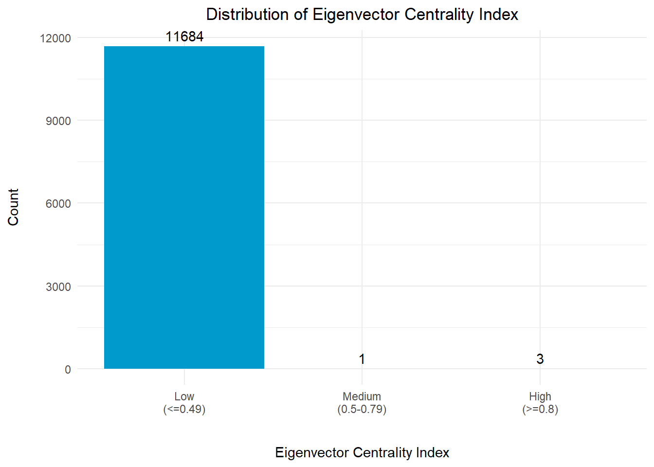
Eigenvector centrality index captures the overall importance of a node based on its connections and the importance of those connections in the network. Nodes with high eigenvector centrality are connected to other nodes that are also highly central or influential.
We will attempt to identify the main hub nodes within the network by looking at the nodes with high eigenvector centrality index.
Firstly, we will take a look at the distribution of this centrality index across all the nodes to gain an overview picture of the network.
Design Considerations
In view of the big differentiation in the count for each bin, the count for each bin is displayed at the top of each bar for easy reference.
# Plotting the Distribution for Eigenvector Centrality Index

# Get the count of the records in each bin
nodes_df_eigen_gp <- nodes_df %>%
  group_by(eigen_bin) %>%
  summarise(cnt = n())

# Create a distribution with bar chart using ggplot2
plot_eigen <- ggplot(nodes_df_eigen_gp, aes(x = eigen_bin, y = cnt)) +
  geom_bar(stat = "identity", fill = "deepskyblue3") +
  geom_text(aes(label = cnt), vjust = -0.5, color = "black") +
  labs(x = "\nEigenvector Centrality Index", y = "Count\n",
       title = "Distribution of Eigenvector Centrality Index") +
  theme_minimal() +
  theme(plot.title = element_text(hjust = 0.5))

plot_eigenThe graph above revealed that there are 4 nodes with eigenvector centrality index of >0.5. This means that these nodes are likely to be connected to other important nodes in the network.
A quick examination of the eigenvector centrality index of the nodes revealed that 11,657 out of 11,688 nodes (>99%) have an eigenvector centrality index of <0.1. Hence, for the purpose of visual analysis, we will just focus on these 4 nodes and the connectivity between its immediate neighbouring nodes.
We will take a closer look at the in-degree centrality index and out-degree centrality index for these 4 nodes which have high eigenvector centrality indices.
# Extracting the top 4 entities with highest centrality indices
nodes_df_eigen_top4 <- nodes_df %>%
  filter(eigen_score >= 0.5) %>%
  select(id, label, eigen_score, eigen_bin, in_degree, in_bin,
         out_degree, out_bin) %>%
  arrange(desc(eigen_score))

datatable(nodes_df_eigen_top4,
          class="stripe",
          caption = "\nTable 1: Business Entities with High Eigenvector Centrality Index\n",
          colnames = c("ID", "Entity", "Eigenvector Centrality Index",
                       "Eigenvector Centrality Category",
                       "In-Degree Centrality Index",
                       "In-Degree Centrality Category",
                       "Out-Degree Centrality Index",
                       "Out-Degree Centrality Category"),
          options = list(
            columnDefs = list(list(className = 'dt-center',
targets="_all"))))Based on the information presented in Table 1 above, we observed that these 4 nodes also have very high number of in-degree centrality index and very low number of out-degree centrality index, suggesting that they are likely to be the transhipments/fishery wharves/central collection centers within the network.
# get the company names for the edges
edges_df_eigen <- edges_df %>%
  filter(from %in% nodes_df_eigen_top4$id |
         to %in% nodes_df_eigen_top4$id) %>%
  filter(weight > 50)

# build the nodes table
nodes_eigen <- nodes_df %>%
  filter(id %in% c(edges_df_eigen$from, edges_df_eigen$to)) %>%
  rename(group = eigen_bin) %>%
  arrange(label)


visNetwork(nodes_eigen,
           edges_df_eigen,
           main = "Network Graph of the Top 4 Entities with High Eigenvector Centrality") %>%
  visIgraphLayout(layout = "layout_with_fr") %>%
  visLayout(randomSeed = 1234) %>%
  visOptions(highlightNearest = list(enabled = T, degree = 2, hover = T),
             nodesIdSelection = TRUE) %>%
  visNodes(id = nodes_eigen$id, size=50) %>%
  visLegend(width = 0.1, position = "right", main = "Group") %>%
  visEdges(arrows = "to",
           smooth = list(enabled = TRUE,
type = "curvedCW"))The Network Graph revealed that all the links to the 4 high eigenvector centrality nodes were in-flow from external nodes. This reaffirms the suggestion that these nodes are likely to be the transhipments/fishery wharves/central collection centers within the network.
Degree centrality is a measure of the importance or popularity of a node in a network based on the number of direct connections it has with other nodes in the network.

# Plotting the Distribution for Degree Centrality Index
nodes_df_deg_gp <- nodes_df %>%
  group_by(deg_bin) %>%
  summarise(cnt = n())

# Create a bar chart with hover text using ggplot2
plot <- ggplot(nodes_df_deg_gp, aes(x = deg_bin, y = cnt)) +
  geom_bar(stat = "identity", fill = "deepskyblue3") +
  geom_text(aes(label = cnt), vjust = -0.5, color = "black") +
  labs(x = "\nDegree Centrality", y = "Count\n",
       title = "Distribution of Degree Centrality of the Nodes") +
  theme_minimal() +
  theme(plot.title = element_text(hjust = 0.5))

plotThe distribution chart above revealed that more than 99% of the nodes have low degree centrality index. There are 18 nodes with high degree centrality index of >= 300. This means that these nodes have significantly high number of direct connections to other nodes within the network.
We will take a look at the different centrality indices for these 18 nodes.
# Extract the nodes with high degree centrality index

nodes_df_deg <- nodes_df %>%
  filter(degree_score >= 300) %>%
  select(id, label, degree_score, deg_bin,
         in_degree, in_bin, out_degree, out_bin) %>%
  arrange(desc(degree_score))

datatable(nodes_df_deg,
          class="stripe",
          caption = "\nTable 2: Business Entities with High Degree Centrality Index\n",
          colnames = c("ID", "Entity",
                       "Degree Centrality Index",
                       "Degree Centrality Category",
                       "In-Degree Centrality Index",
                       "In-Degree Centrality Category",
                       "Out-Degree Centrality Index",
                       "Out-Degree Centrality Category"),
          options = list(
            columnDefs = list(list(className = 'dt-center',
targets="_all"))))Based on the information presented in Table 2 above, we observed that these nodes with high degree centrality indicdes also have very high number of out-degree centrality index. In addition, majority of these nodes also have some incoming links from the other external nodes, suggesting that these nodes would likely to be transhipments within the network.
# get the entity names for the edges
edges_df_deg <- edges_df %>%
  filter(from %in% nodes_df_deg$id |
         to %in% nodes_df_deg$id) %>%
  filter(weight > 30)

# build the nodes table
nodes_deg <- nodes_df %>%
  filter(id %in% c(edges_df_deg$from, edges_df_deg$to)) %>%
  rename(group = deg_bin) %>%
  arrange(label)

visNetwork(nodes_deg,
           edges_df_deg,
           main = "Entities with High Degree Centrality Index") %>%
  visIgraphLayout(layout = "layout_with_kk") %>%
  visLayout(randomSeed = 1234) %>%
  visOptions(highlightNearest = list(enabled = T, degree = 2, hover = T),
             nodesIdSelection = TRUE) %>%
  visNodes(id = nodes_deg$id, size=30) %>%
  visLegend(width = 0.1, position = "right", main = "Group") %>%
  visEdges(arrows = "to",
smooth = list(enabled = TRUE))We observed that the nodes with high degree centrality index (in yellow) generally have outgoing connections to other nodes, which suggested that these nodes are likely to be the bigger fishing vessels or transhipments. Particularly, 2 of these nodes (The Salty Dog Limited Liability Company and xiǎo xiā Oyj Marine ecology) also have incoming links to them.
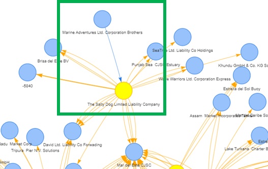
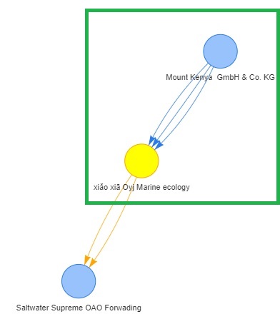
Given that illegal fishing at international waters would typically involve large vessels acting as transhipments to ‘launder’ the illegally caught fish by exchanging for other resources such as fuel, we will examine the hscodes that these 2 entities have, as part of investigation.
We will extract out all the non-fishing related hscodes that involve this company as the source and target to further understand what are the resources that were being traded with the other entities. Once we extracted the relevant records, we will do a count of the number of edges with n() and analyse the top 10 records with the highest number of count.
## Salty Dog as the Source
# Extract all the list of hscodes from the original list of edges (i.e. mc2_edges)
salty_dog_source_details <- mc2_edges %>%
  filter(source == "The Salty Dog Limited Liability Company") %>%
  filter(source != target) %>%
  group_by(target, weightkg, hscode, year) %>%
  summarise(weight = n()) %>%
  distinct() %>%
  ungroup()

# Extract the non-fishing related hscodes and year; and
# sort the records by the weight in descending order
salty_dog_source_hscodes <- salty_dog_source_details %>%
  filter(!(substr(hscode, 1, 3) %in% rel_hscodes_3) &
         !(substr(hscode, 1, 4) %in% rel_hscodes_4)) %>%
  group_by(weightkg, hscode, year, weight) %>%
  distinct() %>%
  arrange(desc(weight)) %>%
  ungroup()


## Salty Dog as the Target
# Extract all the list of hscodes from the original list of edges (i.e. mc2_edges)
salty_dog_target_details <- mc2_edges %>%
  filter(target == "The Salty Dog Limited Liability Company") %>%
  filter(source != target) %>%
  group_by(source, weightkg, hscode, year) %>%
  summarise(weight = n()) %>%
  arrange(desc(weight)) %>%
  distinct() %>%
  ungroup()


# Extract the non-fishing related hscodes and year; and
# sort the records by the weight in descending order
salty_dog_target_hscodes <- salty_dog_target_details %>%
  filter(!(substr(hscode, 1, 3) %in% rel_hscodes_3) &
         !(substr(hscode, 1, 4) %in% rel_hscodes_4)) %>%
  group_by(weightkg, hscode, year, weight) %>%
  distinct() %>%
  arrange(desc(weight)) %>%
  ungroup()


# Presenting the top 10 records in a data table (Source) for analysis
datatable(head(salty_dog_source_hscodes,10),
          class="stripe",
          caption = "\nTable 3: List of Business Entities with 'Salty Dog' as the Source\n",
          colnames = c("Target Entity", "Weightkg",
                       "HS Code", "Year", "Count"),
          options = list(
            columnDefs = list(list(className = 'dt-center',
targets="_all"))))# Presenting the top 10 records in a data table (Target) for analysis
datatable(head(salty_dog_target_hscodes,10),
class="stripe",
caption = "\nTable 4: List of Business Entities with 'Salty Dog' as the Target\n",
colnames = c("Source Entity", "Weightkg", "HS Code",
"Year", "Count"),
options = list(
columnDefs = list(list(className = 'dt-center',
targets="_all"))))Salty Dog as the Source Provider
Table 3 shows that list of Business Entities with ‘Salty Dog’ as the Source Provider. From the list of HS Codes, we noted that ‘The Salty Dog Limited Liability Company’ also provides other forms of consumables, particularly vegetables (for hscodes starting with 710 to 713) to the respective parties. Based on the value of the Count column for these products, we conclude that the trades were unlikely to be related to IUU fishing.
Salty Dog as the Target Recipient
Table 4 shows the list of Business Entities with ‘Salty Dog’ as the Target Recipient. From the list of HS Codes, we noticed that ‘The Salty Dog Limited Liability Company’ does not only accept fish and seafood, but also other products such as bags, container cases/boxes with outer surface of plastics or of textile materials (for hscode == 420212). However, given that the values of the Count column were not extremely high, we conclude that the trades were unlikely to be related to IUU fishing.
Similarly for the close examination of “xiǎo xiā Oyj Marine ecology”, we will extract out all the non-fishing related hscodes that involve this company as the source and target to further understand what are the resources that were being traded with the other entities. Once we extracted the relevant records, we will do a count of the number of edges with n() and analyse the top 10 records with the highest number of count.
## xiǎo xiā as the Source
# Extract all the list of hscodes from the original list of edges (i.e. mc2_edges)
xiao_xia_source_details <- mc2_edges %>%
  filter(source == "xiǎo xiā Oyj Marine ecology") %>%
  filter(source != target) %>%
  group_by(target, weightkg, hscode, year) %>%
  summarise(weight = n()) %>%
  distinct() %>%
  ungroup()

# Extract the non-fishing related hscodes and year; and
# sort the records by the weight in descending order
xiao_xia_source_hscodes <- xiao_xia_source_details %>%
  filter(!(substr(hscode, 1, 3) %in% rel_hscodes_3) &
         !(substr(hscode, 1, 4) %in% rel_hscodes_4)) %>%
  group_by(weightkg, hscode, year, weight) %>%
  distinct() %>%
  arrange(desc(weight)) %>%
  ungroup()


## xiǎo xiā as the Target
# Extract all the list of hscodes from the original list of edges (i.e. mc2_edges)
xiao_xia_target_details <- mc2_edges %>%
  filter(target == "xiǎo xiā Oyj Marine ecology") %>%
  filter(source != target) %>%
  group_by(source, weightkg, hscode, year) %>%
  summarise(weight = n()) %>%
  arrange(desc(weight)) %>%
  distinct() %>%
  ungroup()


# Extract the non-fishing related hscodes and year; and
# sort the records by the weight in descending order
xiao_xia_target_hscodes <- xiao_xia_target_details %>%
  filter(!(substr(hscode, 1, 3) %in% rel_hscodes_3) &
         !(substr(hscode, 1, 4) %in% rel_hscodes_4)) %>%
  group_by(weightkg, hscode, year, weight) %>%
  distinct() %>%
  arrange(desc(weight)) %>%
  ungroup()


# Presenting the top 10 records in a data table (Source) for analysis
datatable(head(xiao_xia_source_hscodes, 10),
          class="stripe",
          caption = "\nTable 5: List of Business Entities with 'Xiao Xia' as the Source\n",
          colnames = c("Target Entity", "Weightkg", "HS Code",
                       "Year", "Count"),
          options = list(
            columnDefs = list(list(className = 'dt-center',
targets="_all"))))# Presenting the top 10 records in a data table (Target) for analysis
datatable(head(xiao_xia_target_hscodes, 10),
class="stripe",
caption = "\nTable 6: List of Business Entities with 'Xiao Xia' as the Target\n",
colnames = c("Source Entity", "Weightkg", "HS Code",
"Year", "Count"),
options = list(
columnDefs = list(list(className = 'dt-center',
targets="_all"))))xiǎo xiā as the Source Provider
Table 5 shows that list of Business Entities with ‘xiǎo xiā’ as the Source Provider. From the list of HS Codes, we noted that ‘xiǎo xiā Oyj Marine ecology’ also provides other products such as:
hscode == 851220)hscode == 390720)hscode == 680293). Based on the value of the Count column for these products, we conclude that the trades were unlikely to be related to IUU fishing.xiǎo xiā as the Target Recipient
Table 6 shows the list of Business Entities with ‘xiǎo xiā’ as the Target Recipient. From the list of HS Codes, we noticed that ‘xiǎo xiā Oyj Marine ecology’ does not only accept fish and seafood, but printed paper or paperboard labels (for hscode = 482110) among the others. However, given that the values of the Count column were not extremely high, we conclude that the trades were unlikely to be related to IUU fishing.
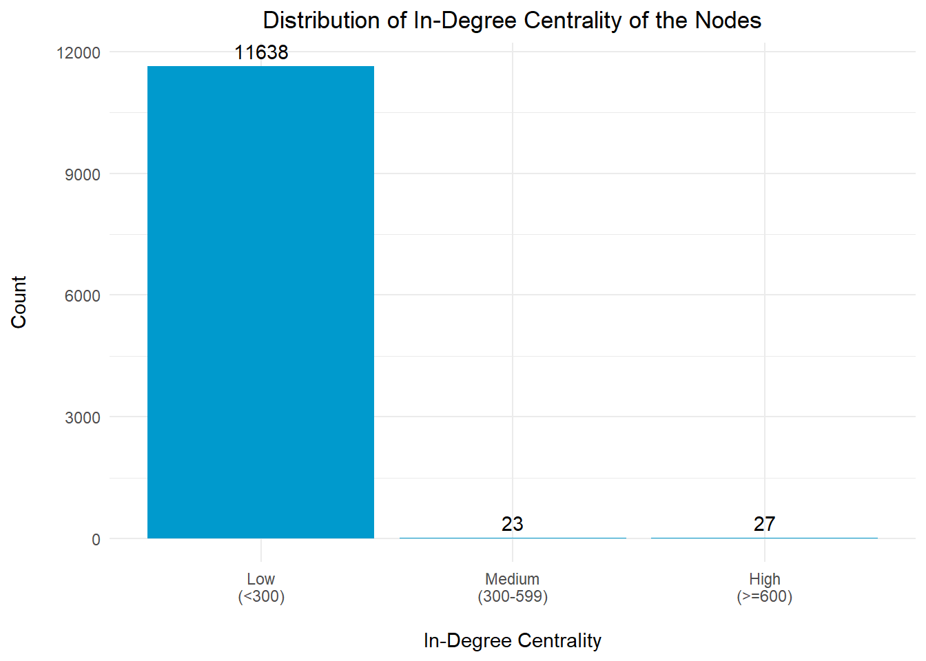
In-degree centrality is another measure of centrality in a network that focuses on incoming connections to a node. Nodes with high in-degree centrality have a larger number of connections pointing towards them, indicating that they receive a lot of resources from other nodes.
# Plotting the Distribution for In-Degree centrality Index
nodes_df_in <- nodes_df %>%
  group_by(in_bin) %>%
  summarise(cnt = n())

# Create a bar chart with hover text using ggplot2
plot_in <- ggplot(nodes_df_in, aes(x = in_bin, y = cnt)) +
  geom_bar(stat = "identity", fill = "deepskyblue3") +
  geom_text(aes(label = cnt), vjust = -0.5, color = "black") +
  labs(x = "\nIn-Degree Centrality", y = "Count\n",
       title = "Distribution of In-Degree Centrality of the Nodes") +
  theme_minimal() +
  theme(plot.title = element_text(hjust = 0.5))

plot_inIt is observed that there are 27 nodes with significantly high in-degree centrality index (>=600), which are likely to be transhipments/collection hubs for the fishing vessels.
For the purpose of analysis, we will focus on the top 10 entities that have the highest in-degree centrality indices.
# Extracting the top 10 entities with highest in-degree centrality
nodes_df_in_top <- nodes_df %>%
  filter(in_degree >= 600) %>%
  select(id, label, in_degree, in_bin,
         eigen_score, eigen_bin, out_degree, out_bin) %>%
  arrange(desc(in_degree))

top_10_in <- head(nodes_df_in_top,10)

datatable(top_10_in,
          class="stripe",
          caption = "\nTable 7: Top 10 Business Entities with High In-Degree Centrality Index\n",
          colnames = c("ID", "Entity", "In-Degree Centrality Index",
                       "In-Degree Centrality Category",
                       "Eigenvector Centrality Index",
                       "Eigenvector Centrality Category",
                       "Out-Degree Centrality Index",
                       "Out-Degree Centrality Category"),
          options = list(
            columnDefs = list(list(className = 'dt-center',
targets="_all"))))It is noted that the 4 entities that have high eigenvector centrality indices in Section 4.2.2. are also listed in Table 7 above. This confirms our earlier suggestion that these nodes are likely to be key transhipments (main collection centres) for the fishing vessels within the network.
# get the entity names for the edges
edges_df_in <- edges_df %>%
  filter(from %in% top_10_in$id |
         to %in% top_10_in$id) %>%
  filter(weight > 80)

# build the nodes table
nodes_in <- nodes_df %>%
  filter(id %in% c(edges_df_in$from, edges_df_in$to)) %>%
  rename(group = in_bin) %>%
  arrange(label)

visNetwork(nodes_in,
           edges_df_in,
           main = "Entities with High In-Degree Centrality Index") %>%
  visIgraphLayout(layout = "layout_with_fr") %>%
  visLayout(randomSeed = 1234) %>%
  visOptions(highlightNearest = list(enabled = T, degree = 2, hover = T),
             nodesIdSelection = TRUE) %>%
  visNodes(id = nodes_in$id, size=30) %>%
  visLegend(width = 0.1, position = "right", main = "Group") %>%
  visEdges(arrows = "to",
           smooth = list(enabled = TRUE,
type = "curvedCW"))The Network Graph above reaffirms that these nodes are likely to be the transhipments for the fishing vessels, in view of the number of incoming links to them.
The graph above also highlighted one of the source provider nodes, “Adriatic Tuna Seabass BV Transit”, has a moderately high value of in-degree centrality index (the node in red).
As part of a close examination of “Adriatic Tuna Seabass BV Transit”, we will extract out all the non-fishing related hscodes that involve this company as the source and target to further understand what are the resources that were being traded with the other entities. Once we extracted the relevant records, we will do a count of the number of edges with n() and analyse the top 10 records with the highest number of count.
## Adriatic as the Source
# Extract all the list of hscodes from the original list of edges (i.e. mc2_edges)
adriatic_source_details <- mc2_edges %>%
  filter(source == "Adriatic Tuna Seabass BV Transit") %>%
  filter(source != target) %>%
  group_by(target, weightkg, hscode, year) %>%
  summarise(weight = n()) %>%
  distinct() %>%
  ungroup()

# Extract the non-fishing related hscodes and year; and
# sort the records by the weight in descending order
adriatic_source_hscodes <- adriatic_source_details %>%
  filter(!(substr(hscode, 1, 3) %in% rel_hscodes_3) &
         !(substr(hscode, 1, 4) %in% rel_hscodes_4)) %>%
  group_by(weightkg, hscode, year, weight) %>%
  distinct() %>%
  arrange(desc(weight)) %>%
  ungroup()


## Adriatic as the Target
# Extract all the list of hscodes from the original list of edges (i.e. mc2_edges)
adriatic_target_details <- mc2_edges %>%
  filter(target == "Adriatic Tuna Seabass BV Transit") %>%
  filter(source != target) %>%
  group_by(source, weightkg, hscode, year) %>%
  summarise(weight = n()) %>%
  arrange(desc(weight)) %>%
  distinct() %>%
  ungroup()


# Extract the non-fishing related hscodes and year; and
# sort the records by the weight in descending order
adriatic_target_hscodes <- adriatic_target_details %>%
  filter(!(substr(hscode, 1, 3) %in% rel_hscodes_3) &
         !(substr(hscode, 1, 4) %in% rel_hscodes_4)) %>%
  group_by(weightkg, hscode, year, weight) %>%
  distinct() %>%
  arrange(desc(weight)) %>%
  ungroup()


# Presenting the top 10 records in a data table (Source) for analysis
datatable(head(adriatic_source_hscodes, 10),
          class="stripe",
          caption = "\nTable 8: List of Business Entities with 'Adriatic' as the Source\n",
          colnames = c("Target Entity", "Weightkg", "HS Code",
                       "Year", "Count"),
          options = list(
            columnDefs = list(list(className = 'dt-center',
targets="_all"))))# Presenting the top 10 records in a data table (Target) for analysis
datatable(head(adriatic_target_hscodes, 10),
class="stripe",
caption = "\nTable 9: List of Business Entities with 'Adriatic' as the Target\n",
colnames = c("Source Entity", "Weightkg", "HS Code",
"Year", "Count"),
options = list(
columnDefs = list(list(className = 'dt-center',
targets="_all"))))Adriatic as the Source Provider
Table 8 shows that list of Business Entities with ‘Adriatic’ as the Source Provider. From the list of HS Codes, we noted that ‘Adriatic Tuna Seabass BV Transit’ also provides other forms of consumables, particularly beancurd related products (for hscode == 210690) and mixtures of fruits, nuts and other edible parts of plants (for hscode == 200897). Based on the value of the Count column for these products, we conclude that the trades were unlikely to be related to IUU fishing.
Adriatic as the Target Recipient
Table 9 shows the list of Business Entities with ‘Adriatic’ as the Target Recipient. From the list of HS Codes, we noticed that ‘Adriatic Tuna Seabass BV Transit’ trades for a moderately high amount of pasta products (for hscode == 190219) and tableware and kitchenware products (for hscode == 848210). However, given that the values of the Count column were not extremely high, we conclude that the trades were unlikely to be related to IUU fishing.
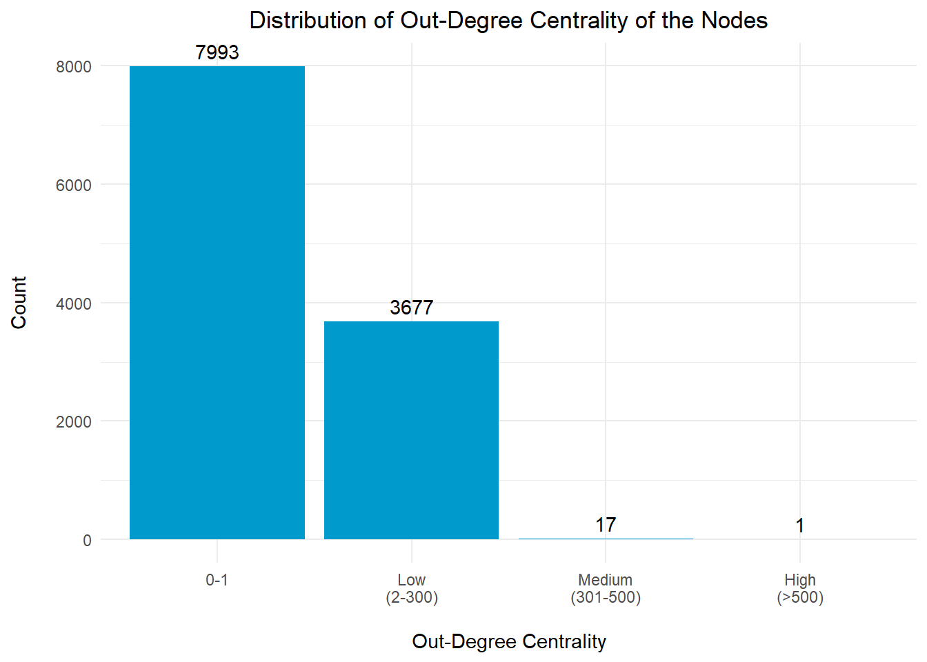
Out-degree centrality is a measure of centrality in a network that focuses on outgoing connections from a node. Nodes with high out-degree centrality have a larger number of connections pointing away from them, indicating that they have a greater reach and influence over other nodes.
# Plotting the Distribution for Out-Degree Centrality Index
nodes_df_out <- nodes_df %>%
  group_by(out_bin) %>%
  summarise(cnt = n())

# Create a bar chart with hover text using ggplot2
plot_in <- ggplot(nodes_df_out, aes(x = out_bin, y = cnt)) +
  geom_bar(stat = "identity", fill = "deepskyblue3") +
  geom_text(aes(label = cnt), vjust = -0.5, color = "black") +
  labs(x = "\nOut-Degree Centrality", y = "Count\n",
       title = "Distribution of Out-Degree Centrality of the Nodes") +
  theme_minimal() +
  theme(plot.title = element_text(hjust = 0.5))

plot_inMajority of the entities (99.8%) in the network have low number of out-degree centrality index, which suggest that they are likely to be the fishing vessels within the network, contributing to one of the major transhipment/fishery wharves/collection centres.
It is observed that there are 18 nodes with significantly high out-degree centrality index (>300), which we will study the top 10 nodes in more details.
# Extracting the top companies with highest out-degree centrality
nodes_df_out <- nodes_df %>%
  filter(out_degree > 300) %>%
  select(id, label, out_degree, out_bin, degree_score, deg_bin,
         betweenness_score, bet_bin) %>%
  arrange(desc(out_degree))

top_10_out <- head(nodes_df_out,10)

datatable(top_10_out,
          class="stripe",
          caption = "\nTable 10: Top 10 Business Entities with High Out-Degree Centrality Index\n",
          colnames = c("ID", "Entity", "Out-Degree Centrality Index",
                       "Out-Degree Centrality Category",
                       "Degree Centrality Index",
                       "Degree Centrality Category",
                       "Betweenness Centrality Index",
                       "Betweenness Centrality Category"),
          options = list(
            columnDefs = list(list(className = 'dt-center',
targets="_all"))))It is observed that the top 10 entities with high value of out-degree centrality index, have a high value for degree centrality and 2 of them also have a high value for betweenness centrality index. This suggested that these 2 entities (“The Salty Dog Limited Liability Company” and “Aqua Aura SE Marine life”) are likely to be the primary transhipment hubs within the network.
# get the company names for the edges
edges_df_out <- edges_df %>%
  filter(from %in% top_10_out$id |
         to %in% top_10_out$id) %>%
  filter(weight > 30)

# build the nodes table
nodes_out <- nodes_df %>%
  filter(id %in% c(edges_df_out$from, edges_df_out$to)) %>%
  rename(group = out_bin) %>%
  arrange(label)

visNetwork(nodes_out,
           edges_df_out,
           main = "Entities with High Out-Degree Centrality Index") %>%
  visIgraphLayout(layout = "layout_with_fr") %>%
  visLayout(randomSeed = 1234) %>%
  visOptions(highlightNearest = list(enabled = T, degree = 2, hover = T),
             nodesIdSelection = TRUE) %>%
  visNodes(id = nodes_out$id, size=30) %>%
  visLegend(width = 0.1, position = "right", main = "Group") %>%
  visEdges(arrows = "to",
           smooth = list(enabled = TRUE,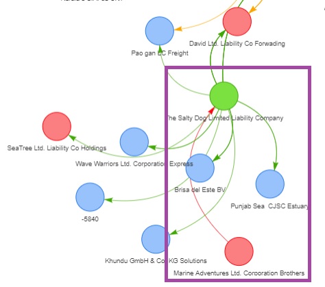
type = "curvedCW"))It is observed that while most of the nodes in this top 10 entities with high out-degree centrality indices, only have outgoing connections to the external nodes, the #1 entity at the top of the list, “The Salty Dog Limited Liability Company”, actually has an incoming connection from another node, “Marine Adventures Ltd. Corporation Brothers”. Hence, we will take a closer look at the exchanges between them.
We will first of all, extract out all the exchanges between “Marine Adventures Ltd. Corporation Brothers” and “The Salty Dog Limited Liability Company”, that do not fall under the fishing related hscodes and perform a closer examination of the other products (if any) that these 2 entities are trading.
## Marine Adventures as the Source and Salty Dog as the Target
# Extract all the non-fishing related hscodes from the original list of edges (i.e. mc2_edges)
marine_source_details <- mc2_edges %>%
  filter(source == "Marine Adventures Ltd. Corporation Brothers" &
         target == "The Salty Dog Limited Liability Company") %>%
  filter(!(substr(hscode, 1, 3) %in% rel_hscodes_3) &
         !(substr(hscode, 1, 4) %in% rel_hscodes_4)) %>%
  group_by(weightkg, hscode, year) %>%
  summarise(weight = n()) %>%
  distinct() %>%
  ungroup()

marine_source_details
# A tibble: 0 × 4
# ℹ 4 variables: weightkg <int>, hscode <chr>, year <dbl>, weight <int>Based on the results, it is concluded that ‘Marine Adventures Ltd. Corporation Brothers’ and ‘The Salty Dog Limited Liability Company’ do not trade any other products that are not related to fishing.
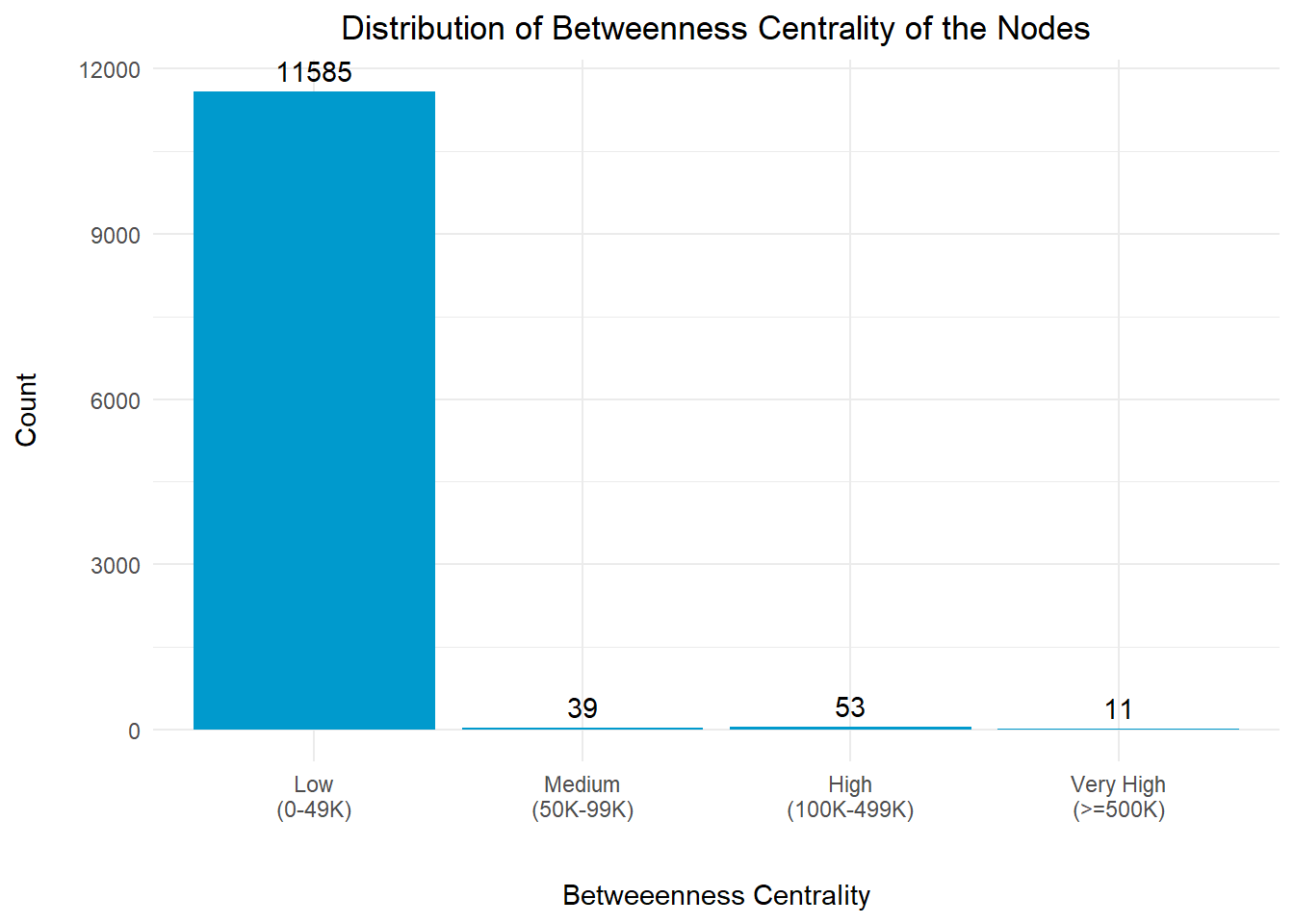
Betweenness centrality is a measure of the importance or influence of a node in a network based on its ability to connect other nodes. Nodes with high betweenness centrality act as bridges or intermediaries, connecting different parts of the network and have the potential to control the flow of information or influence within the network.
In the context of this exercise, nodes with high betweenness centrality might potentially be impact the network.
# Get the count of the records in each bin
nodes_df_bet_gp <- nodes_df %>%
  group_by(bet_bin) %>%
  summarise(cnt = n())

# Create a distribution with bar chart using ggplot2
plot_bet <- ggplot(nodes_df_bet_gp, aes(x = bet_bin, y = cnt)) +
  geom_bar(stat = "identity", fill = "deepskyblue3") +
  geom_text(aes(label = cnt), vjust = -0.5, color = "black") +
  labs(x = "\nBetweeenness Centrality", y = "Count\n",
       title = "Distribution of Betweenness Centrality of the Nodes") +
  theme_minimal() +
  theme(plot.title = element_text(hjust = 0.5))

plot_bet
The betweenness centrality distribution revealed that a large number of nodes has a low value and might potentially be the fishing vessels or small clusters without much influence to the entire network.
However, it is noted that there are 11 nodes with very high betweenness centrality index (>=500K), and we should take a closer look at them to understand their relationships with the other nodes.
For the purpose of analysis, we will focus on the top 11 entities that have the highest betweenness centrality indices.
# Extract the Top 11 nodes with extremely high betweenness centrality index

nodes_df_bet_top11 <- nodes_df %>%
  filter(betweenness_score >= 500000) %>%
  select(id, label, betweenness_score, bet_bin,
         in_degree, in_bin, out_degree, out_bin) %>%
  arrange(desc(betweenness_score))

datatable(nodes_df_bet_top11,
          class="stripe",
          caption = "\nTable 11: Top 11 Business Entities with High Betweenness Centrality Index\n",
          colnames = c("ID", "Entity", "Betweenness Centrality Index",
                       "Betweenness Centrality Category", "In-Degree Centrality Index",
                       "In-Degree Centrality Category", "Out-Degree Centrality Index",
                       "Out-Degree Centrality Cateogy"),
          options = list(
columnDefs = list(list(className = 'dt-center', targets = "_all"))))Table 11 above revealed that 10 out of the 11 entities have low values for their in-degree and out-degree centrality indices.
‘David Ltd. Liability Co Forwading’ is the only entity with a h in-degree centrality index that is in the medium range of (300-599). We will take a closer look at this.
# get the entity names for the edges
edges_df_bet <- edges_df %>%
  filter(from %in% nodes_df_bet_top11$id |
         to %in% nodes_df_bet_top11$id) %>%
  filter(weight > 20)

# build the nodes table
nodes_bet <- nodes_df %>%
  filter(id %in% c(edges_df_bet$from, edges_df_bet$to)) %>%
  rename(group = bet_bin) %>%
  arrange(label)

visNetwork(nodes_bet,
           edges_df_bet,
           main = "Entities with High Betweeness Centrality Index") %>%
  visIgraphLayout(layout = "layout_with_kk") %>%
  visLayout(randomSeed = 1234) %>%
  visOptions(highlightNearest = list(enabled = T, degree = 2, hover = T),
             nodesIdSelection = TRUE) %>%
  visNodes(id = nodes_bet$id, size=30) %>%
  visLegend(width = 0.1, position = "right", main = "Group") %>%
  visEdges(arrows = "to",
smooth = list(enabled = TRUE))The network graph above shows that there are 2 big clusters of nodes.
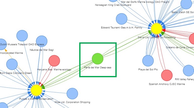
The image above shows that ‘Perla del Mar Deep-sea’ is the key node that connects the 2 nodes (‘Punjab s Marine Conservation’ and ‘David Ltd. Liability Co Forwading’) with high betweenness indices.
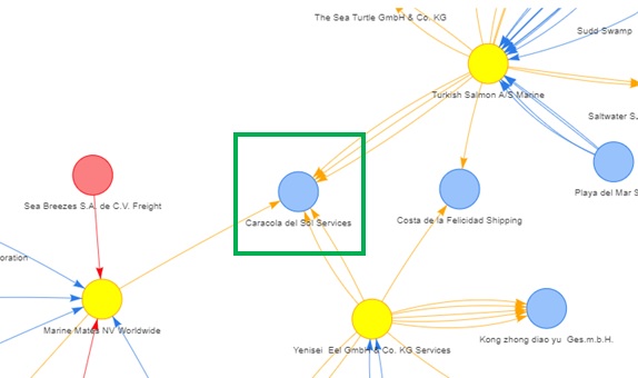
The second image shows that ‘Caracola del Sol Services’ is the key node that connects the 3 nodes (‘Marine Mates NV Worldwide’, ‘Yenisei Eel GmbH & Co. KG Services’ and ‘Turkish Salmon A/S Marine’) with high betweenness indices.
We will extract out all the non-fishing related hscodes that involve this company as the source and target to further understand what are the resources that were being traded with the other entities. Once we extracted the relevant records, we will do a count of the number of edges with n() and analyse the top 10 records with the highest number of count.
## Perla as the Source
# Extract all the list of hscodes from the original list of edges (i.e. mc2_edges)
perla_source_details <- mc2_edges %>%
  filter(source == "Perla del Mar Deep-sea") %>%
  filter(source != target) %>%
  group_by(target, weightkg, hscode, year) %>%
  summarise(weight = n()) %>%
  distinct() %>%
  ungroup()

# Extract the non-fishing related hscodes and year; and
# sort the records by the weight in descending order
perla_source_hscodes <- perla_source_details %>%
  filter(!(substr(hscode, 1, 3) %in% rel_hscodes_3) &
         !(substr(hscode, 1, 4) %in% rel_hscodes_4)) %>%
  group_by(weightkg, hscode, year, weight) %>%
  distinct() %>%
  arrange(desc(weight)) %>%
  ungroup()


## Perla as the Target
# Extract all the list of hscodes from the original list of edges (i.e. mc2_edges)
perla_target_details <- mc2_edges %>%
  filter(target == "Perla del Mar Deep-sea") %>%
  filter(source != target) %>%
  group_by(source, weightkg, hscode, year) %>%
  summarise(weight = n()) %>%
  arrange(desc(weight)) %>%
  distinct() %>%
  ungroup()


# Extract the non-fishing related hscodes and year; and
# sort the records by the weight in descending order
perla_target_hscodes <- perla_target_details %>%
  filter(!(substr(hscode, 1, 3) %in% rel_hscodes_3) &
         !(substr(hscode, 1, 4) %in% rel_hscodes_4)) %>%
  group_by(weightkg, hscode, year, weight) %>%
  distinct() %>%
  arrange(desc(weight)) %>%
  ungroup()


# Presenting the records in a data table (Source) for analysis
datatable(perla_source_hscodes,
          class="stripe",
          caption = "\nTable 12: List of Business Entities with 'Perla' as the Source\n",
          colnames = c("Target Entity", "Weightkg",
                       "HS Code", "Year", "Count"),
          options = list(
            columnDefs = list(list(className = 'dt-center',
targets="_all"))))# Presenting the top 10 records in a data table (Target) for analysis
datatable(head(perla_target_hscodes,10),
class="stripe",
caption = "\nTable 13: List of Business Entities with 'Perla' as the Target\n",
colnames = c("Source Entity", "Weightkg", "HS Code",
"Year", "Count"),
options = list(
columnDefs = list(list(className = 'dt-center',
targets="_all"))))Perla as the Source Provider
Table 12 shows that list of Business Entities with ‘Perla’ as the Source Provider. From the list of HS Codes, we noted that ‘Perla del Mar Deep-sea’ also provides other variety of products such as rubber pneumatic tyres for tractors, machinery (hscode == 401180) upholstered seats (hscode == 940161) to other entities. Based on the value of the Count column for these products, we conclude that the trades were unlikely to be related to IUU fishing.
Perla as the Target Recipient
Table 13 shows the list of Business Entities with ‘Perla’ as the Target Recipient. From the list of HS Codes, we noticed that ‘Perla del Mar Deep-sea’ does not only accept fish and seafood, but also parts suitable for use solely or principally with spark-ignition internal combustion piston engines (for hscode == 840991) from ‘Costa del Sol Sp’, particularly in Year 2028 and 2029.
We will extract out all the non-fishing related hscodes that involve this company as the source and target to further understand what are the resources that were being traded with the other entities. Once we extracted the relevant records, we will do a count of the number of edges with n() and analyse the top 10 records with the highest number of count.
## Caracola as the Source
# Extract all the list of hscodes from the original list of edges (i.e. mc2_edges)
caracol_source_details <- mc2_edges %>%
  filter(source == "Caracola del Sol Services") %>%
  filter(source != target) %>%
  group_by(target, weightkg, hscode, year) %>%
  summarise(weight = n()) %>%
  distinct() %>%
  ungroup()

# Extract the non-fishing related hscodes and year; and
# sort the records by the weight in descending order
caracol_source_hscodes <- caracol_source_details %>%
  filter(!(substr(hscode, 1, 3) %in% rel_hscodes_3) &
         !(substr(hscode, 1, 4) %in% rel_hscodes_4)) %>%
  group_by(weightkg, hscode, year, weight) %>%
  distinct() %>%
  arrange(desc(weight)) %>%
  ungroup()


## Caracola as the Target
# Extract all the list of hscodes from the original list of edges (i.e. mc2_edges)
caracol_target_details <- mc2_edges %>%
  filter(target == "Caracola del Sol Services") %>%
  filter(source != target) %>%
  group_by(source, weightkg, hscode, year) %>%
  summarise(weight = n()) %>%
  arrange(desc(weight)) %>%
  distinct() %>%
  ungroup()


# Extract the non-fishing related hscodes and year; and
# sort the records by the weight in descending order
caracol_target_hscodes <- caracol_target_details %>%
  filter(!(substr(hscode, 1, 3) %in% rel_hscodes_3) &
         !(substr(hscode, 1, 4) %in% rel_hscodes_4)) %>%
  group_by(weightkg, hscode, year, weight) %>%
  distinct() %>%
  arrange(desc(weight)) %>%
  ungroup()


# Presenting the records in a data table (Source) for analysis
datatable(head(caracol_source_hscodes,10),
          class="stripe",
          caption = "\nTable 14: List of Business Entities with 'Caracola' as the Source\n",
          colnames = c("Target Entity", "Weightkg",
                       "HS Code", "Year", "Count"),
          options = list(
            columnDefs = list(list(className = 'dt-center',
targets="_all"))))# Presenting the top 10 records in a data table (Target) for analysis
datatable(head(caracol_target_hscodes,10),
class="stripe",
caption = "\nTable 15: List of Business Entities with 'Caracola' as the Target\n",
colnames = c("Source Entity", "Weightkg", "HS Code",
"Year", "Count"),
options = list(
columnDefs = list(list(className = 'dt-center',
targets="_all"))))Caracola as the Source Provider
Table 14 shows that list of Business Entities with ‘Caracola’ as the Source Provider. From the list of HS Codes, we noted that ‘Caracola del Sol Services’ also provides other variety of products such as rubber pneumatic tyres for tractors, machinery (hscode == 401180) upholstered seats (hscode == 940161) to other entities. Based on the value of the Count column for these products, we conclude that the trades were unlikely to be related to IUU fishing.
Caracola as the Target Recipient
Table 15 shows the list of Business Entities with ‘Caracola’ as the Target Recipient. From the list of HS Codes, we noticed that ‘Caracola del Sol Services’ does not only accept fish and seafood, but also a significant volumn of other products such as:
hscode == 392390)hscode == 760120).Since these items are not directly linked to IUU fishing activities, we conclude that the trades were unlikely to be related to IUU fishing.
Even though there were no suggested suspicious entities found to be involved in Illegal, Unreported and Unregulated (IUU) fishing, we have managed to identify the key transhipments in the network. It was also revealed that these transhipments do not necessary just receive the catches from the fishing vessels, but they also trade (either as a provider or recipient) other goods/products with these fishing vessels. These were discovered when we performed closer examinations of some of the key business entities identified in Sections 4.3 to 4.6.