In-Class Exercise 04

1. Getting Started

1.1. Installing and Loading the required R Packages

In this exercise using Exam_data, we will be using tidyverse, rstatix, gt and patchwork.

pacman::p_load(tidyverse, rstatix, gt, patchwork)

1.2. Importing Data (Exam_data)

exam_data <- read_csv("data/Exam_data.csv")

1.3. Visualising Normal Distribution

A Q-Q plot (Quantile-Quantile plot) is used to assess whether a set of data points are normally distributed.

if the data is normally distrbuted, the points in a Q-Q plot will lie on a straight diagonal line. Conversely, if the points deviate significantly from the straight diagonal line, then it’s less likely that the data is normally distributed.

The Plot

The Code Chunk

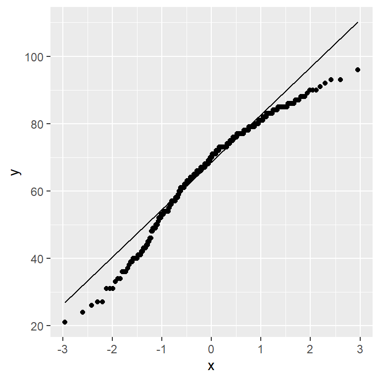
ggplot(exam_data,
       aes(sample=ENGLISH)) + 
  stat_qq() + 
  stat_qq_line()

Note

We can see that the points deviate significantly form the straight diagnoal line. This is a clear indication that the set of data is not normally distributed.

1.4. Runnig Shapiron Test

png, webshot2 packages will be required to run the following codes.

The Plot

The Code Chunk

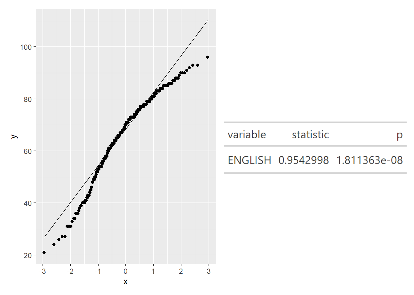
qq <- ggplot(exam_data,
             aes(sample=ENGLISH)) + 
  stat_qq() +
  stat_qq_line()

# running shapiro test and save into gt() format
sw_t <- exam_data %>%
  shapiro_test(ENGLISH) %>%
  gt()


# converting the sw_t into an image file (png)
tmp <- tempfile(fileext = '.png')
gtsave(sw_t, tmp)
table_png <- png::readPNG(tmp,
                          native = TRUE)

qq + table_png